List of modules (API)

blockdata

Module for managing block data (for deesse), and relative functions.

class blockdata.BlockData(blockDataUsage=0, nblock=0, nodeIndex=None, value=None, tolerance=None, activatePropMin=None, activatePropMax=None)

Class defining block data for one variable (for deesse).

Attributes

blockDataUsageint, default: 0

defines the usage of block data:

blockDataUsage=0: no block data
blockDataUsage=1: block data defined as block mean value

nblockint, default: 0

number of block(s) (used if blockDataUsage=1)

nodeIndexsequence of 2D array-like of ints with 3 columns, optional

node index in each block (used if blockDataUsage=1):

nodeIndex[i][j]: sequence of 3 floats, node index in the simulation grid along x, y, z axis of the j-th node of the i-th block

valuesequence of floats of length nblock, optional

target value for each block (used if blockDataUsage=1)

tolerancesequence of floats of length nblock, optional

tolerance for each block (used if blockDataUsage=1)

activatePropMinsequence of floats of length nblock, optional

minimal proportion of informed nodes in the block, under which the block data constraint is deactivated, for each block (used if blockDataUsage=1)

activatePropMaxsequence of floats of length nblock, optional

maximal proportion of informed nodes in the block, above which the block data constraint is deactivated, for each block (used if blockDataUsage=1)

Methods

__init__(blockDataUsage=0, nblock=0, nodeIndex=None, value=None, tolerance=None, activatePropMin=None, activatePropMax=None)

Inits an instance of the class.

Parameters:

blockDataUsage (int, default: 0) – defines the usage of block data
nblock (int, default: 0) – number of block(s)
nodeIndex (sequence of 2D array-like of ints with 3 columns, optional) – node index in each block
value (sequence of floats of length nblock, optional) – target value for each block
tolerance (sequence of floats of length nblock, optional) – tolerance for each block
activatePropMin (sequence of floats of length nblock, optional) – minimal proportion of informed nodes in the block, under which the block data constraint is deactivated, for each block
activatePropMax (sequence of floats of length nblock, optional) – maximal proportion of informed nodes in the block, above which the block data constraint is deactivated, for each block

exception blockdata.BlockDataError: Custom exception related to blockdata module.

blockdata.readBlockData(filename, logger=None)

Reads block data from a txt file.

Parameters:

filename (str) – name of the file
logger (logging.Logger, optional) – logger (see package logging) if specified, messages are written via logger (no print)

Returns:

bd – block data

Return type:

BlockData

blockdata.writeBlockData(bd, filename, fmt='.5g')

Writes block data in a txt file.

Parameters:

bd (BlockData) – block data
filename (str) – name of the file
fmt (str, default: '.5g') – format string for target value, tolerance and active proportion (min and max) in the block data

covModel

Module for:

definition of covariance / variogram models in 1D, 2D, and 3D (omni-directional or anisotropic)
covariance / variogram analysis and fitting
ordinary kriging
cross-validation (leave-one-out (loo))

class covModel.CovModel1D(elem=[], name=None, logger=None)

Class defining a covariance model in 1D.

A covariance model is defined as the sum of elementary covariance models.

An elementary variogram model is defined as its weight parameter (w) minus the covariance elementary model, and a variogram model is defined as the sum of elementary variogram models.

This class is callable, returning the evaluation of the model (covariance or variogram) at given point(s) (lag(s)).

Attributes

elem1D array-like

sequence of elementary model(s) (contributing to the covariance model), each element of the sequence is a 2-tuple (t, d), where

tstr
type of elementary covariance model, can be
- ‘nugget’ (see function cov_nug())
- ‘spherical’ (see function cov_sph())
- ‘exponential’ (see function cov_exp())
- ‘gaussian’ (see function cov_gau())
- ‘triangular’ (see function cov_tri())
- ‘cubic’ (see function cov_cub())
- ‘sinus_cardinal’ (see function cov_sinc())
- ‘gamma’ (see function cov_gamma())
- ‘power’ (see function cov_pow())
- ‘exponential_generalized’ (see function cov_exp_gen())
- ‘matern’ (see function cov_matern())
ddict
dictionary of required parameters to be passed to the elementary model t

e.g.

(t, d) = (‘spherical’, {‘w’:2.0, ‘r’:1.5})
(t, d) = (‘power’, {‘w’:2.0, ‘r’:1.5, ‘s’:1.7})
(t, d) = (‘matern’, {‘w’:2.0, ‘r’:1.5, ‘nu’:1.5})

namestr, optional

name of the model

Private attributes (SHOULD NOT BE SET DIRECTLY)

_rfloat: (effective) range
_sillfloat: sill (sum of weight of elementary contributions)
_is_orientation_stationarybool: indicates if the covariance model has stationary orientation (always True for 1D covariance model)
_is_weight_stationarybool: indicates if the covariance model has stationary weight
_is_range_stationarybool: indicates if the covariance model has stationary range(s)
_is_stationarybool: indicates if the covariance model is stationary

Examples

To define a covariance model (1D) that is the sum of the 2 following elementary models:

gaussian with a contribution (weight) of 10.0 and a range of 100.0,

nugget of (contribution, weight) 0.5

>>> cov_model = CovModel1D(elem=[
    ('gaussian', {'w':10., 'r':100.0}), # elementary contribution
    ('nugget', {'w':0.5})               # elementary contribution
    ], name='gau+nug')                  # name (optional)

Methods

__call__(h, vario=False)

Evaluates the covariance model at given 1D lags (h).

Parameters:

h (1D array-like of floats, or float) – point(s) (lag(s)) where the covariance model is evaluated
vario (bool, default: False) –
- if False: computes the covariance
- if True: computes the variogram

Returns:

y – evaluation of the covariance or variogram model at h; note: the result is casted to a 1D array if h is a float

Return type:

1D array

__init__(elem=[], name=None, logger=None)

Inits an instance of the class.

Parameters:

elem (1D array-like, default: []) – sequence of elementary model(s)
name (str, optional) – name of the model
logger (logging.Logger, optional) – logger (see package logging) if specified, messages are written via logger (no print)

add_w(a, elem_ind=None, logger=None)

Add a`to parameter `w of the (given) elementary contribution(s).

The covariance model is updated and relevant private attributes (beginning with “_”) are reset.

Parameters:

a (array of floats or float) – term(s) to add, if array, its shape must be compatible with the dimension of the grid on which the covariance model is used (for Gaussian interpolation or simulation)
elem_ind (1D array-like of ints, or int, optional) – indexe(s) of the elementary contribution (attribute elem) to be modified; by default (None): indexes of any elementary contribution are selected
logger (logging.Logger, optional) – logger (see package logging) if specified, messages are written via logger (no print)

func()

Returns the function f for the evaluation of the covariance model.

Returns:

f – function with parameters (arguments):

h1D array-like of floats, or float
point(s) (lag(s)) where the covariance model is evaluated

that returns:

f(h)1D array
evaluation of the covariance model at h; note: the result is casted to a 1D array if h is a float

Return type:

function

Notes

No evaluation is done if the model is not stationary (return None).

is_orientation_stationary(recompute=False)

Checks if the covariance model has stationary orientation.

(Always True for 1D covariance model.)

Parameters:: recompute (bool, default: False) – True to force (re-)computing
Returns:: flag – boolean indicating if the orientation is stationary (private attribute _is_orientation_stationary)
Return type:: bool

is_range_stationary(recompute=False)

Checks if the covariance model has stationary range.

Parameters:: recompute (bool, default: False) – True to force (re-)computing
Returns:: flag – boolean indicating if the range (parameter r) of every elementary contribution is stationary (defined as a unique value) (private attribute _is_range_stationary)
Return type:: bool

is_stationary(recompute=False)

Checks if the covariance model is stationary.

Parameters:: recompute (bool, default: False) – True to force (re-)computing
Returns:: flag – boolean indicating if all the parameters are stationary (defined as a unique value) (private attribute _is_stationary)
Return type:: bool

is_weight_stationary(recompute=False)

Checks if the covariance model has stationary weight.

Parameters:: recompute (bool, default: False) – True to force (re-)computing
Returns:: flag – boolean indicating if the weight (parameter w) of every elementary contribution is stationary (defined as a unique value) (private attribute _is_weight_stationary)
Return type:: bool

multiply_r(factor, elem_ind=None, logger=None)

Multiplies parameter r of the (given) elementary contribution(s) by the given factor.

The covariance model is updated and relevant private attributes (beginning with “_”) are reset.

Parameters:

factor (array of floats or float) – multiplier(s), if array, its shape must be compatible with the dimension of the grid on which the covariance model is used (for Gaussian interpolation or simulation)
elem_ind (1D array-like of ints, or int, optional) – indexe(s) of the elementary contribution (attribute elem) to be modified; by default (None): indexes of any elementary contribution are selected
logger (logging.Logger, optional) – logger (see package logging) if specified, messages are written via logger (no print)

multiply_w(factor, elem_ind=None, logger=None)

Multiplies parameter w of the (given) elementary contribution(s) by the given factor.

The covariance model is updated and relevant private attributes (beginning with “_”) are reset.

Parameters:

factor (array of floats or float) – multiplier(s), if array, its shape must be compatible with the dimension of the grid on which the covariance model is used (for Gaussian interpolation or simulation)
elem_ind (1D array-like of ints, or int, optional) – indexe(s) of the elementary contribution (attribute elem) to be modified; by default (None): indexes of any elementary contribution are selected
logger (logging.Logger, optional) – logger (see package logging) if specified, messages are written via logger (no print)

plot_model(vario=False, hmin=0.0, hmax=None, npts=500, show_xlabel=True, show_ylabel=True, grid=True, **kwargs)

Plots the covariance or variogram model f(h) (in the current figure axis).

Parameters:

vario (bool, default: False) –
- if False: plots the covariance
- if True: plots the variogram
hmin (float, default: 0.0) – see hmax
hmax (float, optional) – function is plotted for h in interval [hmin,` hmax`]; by default (hmax=None), hmax is set to 1.2 times the range of the model
npts (int, default: 500) – number of points used in interval [hmin,` hmax`]
show_xlabel (bool, default: True) – indicates if (default) label for abscissa is displayed
show_ylabel (bool, default: True) – indicates if (default) label for ordinate is displayed
grid (bool, default: True) – indicates if a grid is plotted
kwargs (dict) – keyword arguments passed to the funtion matplotlib.pyplot.plot

Notes

No plot is displayed if the model is not stationary.

r(recompute=False)

Retrieves the (effective) range of the covariance model.

The effective range of the model is the maximum of the effective range of all elementary contributions; note that the “effective” range is the distance beyond which the covariance is zero or below 5% of the weight, and corresponds to the parameter r for most of elementary covariance models.

Parameters:: recompute (bool, default: False) – True to force (re-)computing
Returns:: range – (effective) range of the covariance model
Return type:: float

Notes

Nothing is returned if the model has non-stationary range (return None).

reset_private_attributes(): Resets (sets to None) the “private” attributes (beginning with “_”).

sill(recompute=False)

Retrieves the sill of the covariance model.

Parameters:: recompute (bool, default: False) – True to force (re-)computing
Returns:: sill – sill, sum of the weights of all elementary contributions (private attribute _sill)
Return type:: float

Notes

Nothing is returned if the model has non-stationary weight (return None).

vario_func()

Returns the function f for the evaluation of the variogram model.

Returns:

f – function with parameters (arguments):

h1D array-like of floats, or float
point(s) (lag(s)) where the variogram model is evaluated

that returns:

f(h)1D array
evaluation of the variogram model at h; note: the result is casted to a 1D array if h is a float

Return type:

function

Notes

No evaluation is done if the model is not stationary (return None).

class covModel.CovModel2D(elem=[], alpha=0.0, name=None, logger=None)

Class defining a covariance model in 2D.

A covariance model is defined as the sum of elementary covariance models.

An elementary variogram model is defined as its weight parameter (w) minus the covariance elementary model, and a variogram model is defined as the sum of elementary variogram models.

This class is callable, returning the evaluation of the model (covariance or variogram) at given point(s) (lag(s)).

Attributes

elem1D array-like

sequence of elementary model(s) (contributing to the covariance model), each element of the sequence is a 2-tuple (t, d), where

tstr
type of elementary covariance model, can be
- ‘nugget’ (see function cov_nug())
- ‘spherical’ (see function cov_sph())
- ‘exponential’ (see function cov_exp())
- ‘gaussian’ (see function cov_gau())
- ‘triangular’ (see function cov_tri())
- ‘cubic’ (see function cov_cub())
- ‘sinus_cardinal’ (see function cov_sinc())
- ‘gamma’ (see function cov_gamma())
- ‘power’ (see function cov_pow())
- ‘exponential_generalized’ (see function cov_exp_gen())
- ‘matern’ (see function cov_matern())
ddict
dictionary of required parameters to be passed to the elementary model t

e.g.

(t, d) = (‘spherical’, {‘w’:2.0, ‘r’:[1.5, 2.5]})
(t, d) = (‘power’, {‘w’:2.0, ‘r’:[1.5, 2.5], ‘s’:1.7})
(t, d) = (‘matern’, {‘w’:2.0, ‘r’:[1.5, 2.5], ‘nu’:1.5})

alphafloat, default: 0.0

azimuth angle in degrees; the system Ox’y’, supporting the axes of the model (ranges), is obtained from the system Oxy by applying a rotation of angle -alpha. The 2x2 matrix m for changing the coordinates system from Ox’y’ to Oxy is:

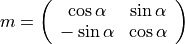
$m = \left(\begin{array}{cc} \cos\alpha & \sin\alpha\\ -\sin\alpha & \cos\alpha \end{array}\right)$

namestr, optional

name of the model

Private attributes (SHOULD NOT BE SET DIRECTLY)

_rfloat: maximal (effective) range, along the two axes
_sillfloat: sill (sum of weight of elementary contributions)
_mrot2D array of shape (2, 2): rotation matrix m (see above)
_is_orientation_stationarybool: indicates if the covariance model has stationary orientation
_is_weight_stationarybool: indicates if the covariance model has stationary weight
_is_range_stationarybool: indicates if the covariance model has stationary range(s)
_is_stationarybool: indicates if the covariance model is stationary

Examples

To define a covariance model (2D) that is the sum of the 2 following elementary models:

gaussian with a contribution (weight) of 10.0 and ranges of 150.0 and 50.0,
nugget of (contribution, weight) 0.5

and in the system Ox’y’ defined by the angle alpha=-30.0

>>> cov_model = CovModel2D(elem=[
        ('gaussian', {'w':10.0, 'r':[150.0, 50.0]}), # elementary contribution
        ('nugget', {'w':0.5})                        # elementary contribution
        ], alpha=-30.0,                              # angle
        name='')                                     # name (optional)

Methods

__call__(h, vario=False)

Evaluates the covariance model at given 2D lags (h).

Parameters:

h (2D array-like of shape (n, 2) or 1D array-like of shape (2,)) – point(s) (lag(s)) where the covariance model is evaluated; if h is a 2D array, each row is a lag
vario (bool, default: False) –
- if False: computes the covariance
- if True: computes the variogram

Returns:

y – evaluation of the covariance or variogram model at h; note: the result is casted to a 1D array if h is a 1D array

Return type:

1D array

__init__(elem=[], alpha=0.0, name=None, logger=None)

Inits an instance of the class.

Parameters:

elem (1D array-like, default: []) – sequence of elementary model(s)
alpha (float, default: 0.0) – azimuth angle in degrees
name (str, optional) – name of the model
logger (logging.Logger, optional) – logger (see package logging) if specified, messages are written via logger (no print)

add_w(a, elem_ind=None, logger=None)

Add a`to parameter `w of the (given) elementary contribution(s).

The covariance model is updated and relevant private attributes (beginning with “_”) are reset.

Parameters:

a (array of floats or float) – term(s) to add, if array, its shape must be compatible with the dimension of the grid on which the covariance model is used (for Gaussian interpolation or simulation)
elem_ind (1D array-like of ints, or int, optional) – indexe(s) of the elementary contribution (attribute elem) to be modified; by default (None): indexes of any elementary contribution are selected
logger (logging.Logger, optional) – logger (see package logging) if specified, messages are written via logger (no print)

func()

Returns the function f for the evaluation of the covariance model.

Returns:

f – function with parameters (arguments):

h2D array-like of shape (n, 2) or 1D array-like of shape (2,)
point(s) (lag(s)) where the covariance model is evaluated; if h is a 2D array, each row is a lag

that returns:

f(h)1D array
evaluation of the covariance model at h; note: the result is casted to a 1D array if h is a 1D array

Return type:

function

Notes

No evaluation is done if the model is not stationary (return None).

is_orientation_stationary(recompute=False)

Checks if the covariance model has stationary orientation.

Parameters:: recompute (bool, default: False) – True to force (re-)computing
Returns:: flag – boolean indicating if the orientation is stationary, i.e. attritbute alpha is defined as a unique value (private attribute _is_orientation_stationary)
Return type:: bool

is_range_stationary(recompute=False)

Checks if the covariance model has stationary ranges.

Parameters:: recompute (bool, default: False) – True to force (re-)computing
Returns:: flag – boolean indicating if the range along each axis (parameter r) of every elementary contribution is stationary (r[i] defined as a unique value) (private attribute _is_range_stationary)
Return type:: bool

is_stationary(recompute=False)

Checks if the covariance model is stationary.

Parameters:: recompute (bool, default: False) – True to force (re-)computing
Returns:: flag – boolean indicating if all the parameters are stationary (defined as a unique value) (private attribute _is_stationary)
Return type:: bool

is_weight_stationary(recompute=False)

Checks if the covariance model has stationary weight.

Parameters:: recompute (bool, default: False) – True to force (re-)computing
Returns:: flag – boolean indicating if the weight (parameter w) of every elementary contribution is stationary (defined as a unique value) (private attribute _is_weight_stationary)
Return type:: bool

mrot(recompute=False)

Returns the 2x2 matrix of rotation defining the axes of the model.

The 2x2 matrix m is the matrix of changes of coordinate system, from Ox’y’ to Oxy, where Ox’ and Oy’ are the axes supporting the ranges of the model.

Parameters:: recompute (bool, default: False) – True to force (re-)computing
Returns:: mrot – rotation matrix (private attribute _mrot)
Return type:: 2D array of shape (2, 2)

Notes

Nothing is returned if the model has non-stationary orientation (return None).

multiply_r(factor, r_ind=None, elem_ind=None, logger=None)

Multiplies (given index(es) of) parameter r of the (given) elementary contribution(s) by the given factor.

The covariance model is updated and relevant private attributes (beginning with “_”) are reset.

Parameters:

factor (array of floats or float) – multiplier(s), if array, its shape must be compatible with the dimension of the grid on which the covariance model is used (for Gaussian interpolation or simulation)
r_ind (int or sequence of ints, optional) – indexe(s) of the parameter r of elementary contribution to be modified; by default (None): r_ind=(0, 1) is used, i.e. parameter r along each axis is multiplied
elem_ind (1D array-like of ints, or int, optional) – indexe(s) of the elementary contribution (attribute elem) to be modified; by default (None): indexes of any elementary contribution are selected
logger (logging.Logger, optional) – logger (see package logging) if specified, messages are written via logger (no print)

multiply_w(factor, elem_ind=None, logger=None)

Multiplies parameter w of the (given) elementary contribution(s) by the given factor.

The covariance model is updated and relevant private attributes (beginning with “_”) are reset.

Parameters:

factor (array of floats or float) – multiplier(s), if array, its shape must be compatible with the dimension of the grid on which the covariance model is used (for Gaussian interpolation or simulation)
elem_ind (1D array-like of ints, or int, optional) – indexe(s) of the elementary contribution (attribute elem) to be modified; by default (None): indexes of any elementary contribution are selected
logger (logging.Logger, optional) – logger (see package logging) if specified, messages are written via logger (no print)

plot_model(vario=False, plot_map=True, plot_curves=True, cmap='terrain', color0='red', color1='green', extent=None, ncell=(201, 201), h1min=0.0, h1max=None, h2min=0.0, h2max=None, n1=500, n2=500, show_xlabel=True, show_ylabel=True, grid=True, show_suptitle=True, figsize=None, logger=None)

Plots the covariance or variogram model.

The model can be displayed as - map of the function, and / or - curves along axis x’ and axis y’ supporting the model.

If map (plot_map=True) and curves (plot_curves=True) are displayed, a new “1x2” figure is used, if only one of map or curves is displayed, the current axis is used.

Parameters:

vario (bool, default: False) –
- if False: the covariance model is displayed
- if True: the variogram model is displayed
plot_map (bool, default: True) – indicates if (2D) map of the model is displayed
plot_curves (bool, default: True) – indicates if curves of the model along x’ and y’ axes are displayed
cmap (colormap) – color map (can be a string, in this case the color map matplotlib.pyplot.get_cmap(cmap)
color0 (color, default: 'red') – color (3-tuple (RGB code), 4-tuple (RGBA code) or str), used for the curve along the 1st axis (x’)
color1 (color, default: 'green') – color (3-tuple (RGB code), 4-tuple (RGBA code) or str), used for the curve along the 2nd axis (y’)
extent (sequence of 4 floats, optional) – extent=(hxmin, hxmax, hymin, hymax) 4 floats defining the limit of the map; by default (extent=None), hxmin, hymin (resp. hxmax, hymax) are set the + (resp. -) 1.2 times max(r1, r2), where r1, r2 are the ranges along the 1st, 2nd axis respectively
ncell (sequence of 2 ints, default: (201, 201)) – ncell=(nx, ny) 2 ints defining the number of the cells in the map along each direction (in “original” coordinates system)
h1min (float, default: 0.0) – see h1max
h1max (float, optional) – function (curve) is plotted for h in interval [h1min,` h1max`] along the 1st axis (x’); by default (h1max=None), h1max is set to 1.2 times max(r1, r2), where r1, r2 are the ranges along the 1st and 2nd axis respectively
h2min (float, default: 0.0) – see h2max
h2max (float, optional) – function (curve) is plotted for h in interval [h2min,` h2max`] along the 2nd axis (y’); by default (h2max=None), h2max is set to 1.2 times max(r1, r2), where r1, r2 are the ranges along the 1st and 2nd axis respectively
n1 (int, default: 500) – number of points for the plot of the curve along the 1st axis, in interval [h1min,` h1max`]
n2 (int, default: 500) – number of points for the plot of the curve along the 2nd axis, in interval [h2min,` h2max`]
show_xlabel (bool, default: True) – indicates if (default) label for abscissa is displayed
show_ylabel (bool, default: True) – indicates if (default) label for ordinate is displayed
grid (bool, default: True) – indicates if a grid is plotted for the plot of the curves
show_suptitle (bool, default: True) – indicates if (default) suptitle is displayed, if both map and curves are plotted (plot_map=True and plot_curves=True) (in a new “1x2” figure)
figsize (2-tuple, optional) – size of the new “1x2” figure, if both map and curves are plotted (plot_map=True and plot_curves=True)
logger (logging.Logger, optional) – logger (see package logging) if specified, messages are written via logger (no print)

Notes

No plot is displayed if the model is not stationary.

plot_model_one_curve(main_axis=1, vario=False, hmin=0.0, hmax=None, npts=500, show_xlabel=True, show_ylabel=True, grid=True, logger=None, **kwargs)

Plots the covariance or variogram curve along one main axis (in the current figure axis).

Parameters:

main_axis (int (1 or 2), default: 1) –
- if main_axis=1, plots the curve along the 1st axis (x’)
- if main_axis=2, plots the curve along the 2nd axis (y’)
vario (bool, default: False) –
- if False: the covariance model is displayed
- if True: the variogram model is displayed
hmin (float, default: 0.0) – see hmax
hmax (float, optional) – function is plotted for h in interval [hmin,` hmax`] along the axis specified by main_axis; by default (hmax=None), hmax is set to 1.2 times the range of the model along the specified axis
npts (int, default: 500) – number of points used in interval [hmin,` hmax`]
show_xlabel (bool, default: True) – indicates if (default) label for abscissa is displayed
show_ylabel (bool, default: True) – indicates if (default) label for ordinate is displayed
grid (bool, default: True) – indicates if a grid is plotted
logger (logging.Logger, optional) – logger (see package logging) if specified, messages are written via logger (no print)
kwargs (dict) – keyword arguments passed to the funtion matplotlib.pyplot.plot

Notes

No plot is displayed if the model is not stationary.

plot_mrot(color0='red', color1='green')

Plots axes of system Oxy and Ox’y’ (in the current figure axis).

Parameters:

color0 (color, default: 'red') – color (3-tuple (RGB code), 4-tuple (RGBA code) or str), used for the 1st axis (x’) supporting the covariance model
color1 (color, default: 'green') – color (3-tuple (RGB code), 4-tuple (RGBA code) or str), used for the 2nd axis (y’) supporting the covariance model

Notes

No plot is displayed if the model has non-stationary orientation.

r12(recompute=False)

Returns the (effective) ranges along x’, y’ axes supporting the model.

The effective range of the model (in a given direction) is the maximum of the effective range of all elementary contributions; note that the “effective” range is the distance beyond which the covariance is zero or below 5% of the weight, and corresponds to the (components of the) parameter r for most of elementary covariance models.

Parameters:: recompute (bool, default: False) – True to force (re-)computing
Returns:: range – (effective) ranges along x’, y’ axes supporting the model (private attribute _r)
Return type:: 1D array of shape (2,)

Notes

Nothing is returned if the model has non-stationary ranges (return None).

reset_private_attributes(): Resets (sets to None) the “private” attributes (beginning with “_”).

rxy(recompute=False)

Returns the (effective) ranges along x, y axes of the “original” coordinates system.

The effective range of the model (in a given direction) is the maximum of the effective range of all elementary contributions; note that the “effective” range is the distance beyond which the covariance is zero or below 5% of the weight, and corresponds to the (components of the) parameter r for most of elementary covariance models.

Parameters:: recompute (bool, default: False) – True to force (re-)computing
Returns:: range – (effective) ranges along x, y axes of the “original” coordinates system
Return type:: 1D array of shape (2,)

Notes

Nothing is returned if the model has non-stationary ranges or non stationary orientation (return None).

set_alpha(alpha)

Sets (modifies) the attribute alpha.

The covariance model is updated and relevant private attributes (beginning with “_”) are reset.

Parameters:: alpha (array of float or float) – azimuth angle in degrees; if array, its shape must be compatible with the dimension of the grid on which the covariance model is used (for Gaussian interpolation or simulation)

sill(recompute=False)

Retrieves the sill of the covariance model.

Parameters:: recompute (bool, default: False) – True to force (re-)computing
Returns:: sill – sill, sum of the weights of all elementary contributions (private attribute _sill)
Return type:: float

Notes

Nothing is returned if the model has non-stationary weight (return None).

vario_func()

Returns the function f for the evaluation of the variogram model.

Returns:

f – function with parameters (arguments):

h2D array-like of shape (n, 2) or 1D array-like of shape (2,)
point(s) (lag(s)) where the variogram model is evaluated; if h is a 2D array, each row is a lag

that returns:

f(h)1D array
evaluation of the variogram model at h; note: the result is casted to a 1D array if h is a 1D array

Return type:

function

Notes

No evaluation is done if the model is not stationary (return None).

class covModel.CovModel3D(elem=[], alpha=0.0, beta=0.0, gamma=0.0, name=None, logger=None)

Class defining a covariance model in 3D.

A covariance model is defined as the sum of elementary covariance models.

An elementary variogram model is defined as its weight parameter (w) minus the covariance elementary model, and a variogram model is defined as the sum of elementary variogram models.

This class is callable, returning the evaluation of the model (covariance or variogram) at given point(s) (lag(s)).

Attributes

elem1D array-like

sequence of elementary model(s) (contributing to the covariance model), each element of the sequence is a 2-tuple (t, d), where

tstr
type of elementary covariance model, can be
- ‘nugget’ (see function cov_nug())
- ‘spherical’ (see function cov_sph())
- ‘exponential’ (see function cov_exp())
- ‘gaussian’ (see function cov_gau())
- ‘triangular’ (see function cov_tri())
- ‘cubic’ (see function cov_cub())
- ‘sinus_cardinal’ (see function cov_sinc())
- ‘gamma’ (see function cov_gamma())
- ‘power’ (see function cov_pow())
- ‘exponential_generalized’ (see function cov_exp_gen())
- ‘matern’ (see function cov_matern())
ddict
dictionary of required parameters to be passed to the elementary model t

e.g.

(t, d) = (‘spherical’, {‘w’:2.0, ‘r’:[1.5, 2.5, 3.0]})
(t, d) = (‘power’, {‘w’:2.0, ‘r’:[1.5, 2.5, 3.0], ‘s’:1.7})
(t, d) = (‘matern’, {‘w’:2.0, ‘r’:[1.5, 2.5, 3.0], ‘nu’:1.5})

alpha, beta, gamma: floats, default: 0.0, 0.0, 0.0

azimuth, dip and plunge angles in degrees; the system Ox’’’y’’’’z’’’, supporting the axes of the model (ranges), is obtained from the system Oxyz as follows:

# Oxyz      -- rotation of angle -alpha around Oz  --> Ox'y'z'
# Ox'y'z'   -- rotation of angle -beta  around Ox' --> Ox''y''z''
# Ox''y''z''-- rotation of angle -gamma around Oy''--> Ox'''y'''z'''

The 3x3 matrix m for changing the coordinates system from Ox’’’y’’’z’’’ to Oxyz is:

$m = \left(\begin{array}{rrr} \cos\alpha \cdot \cos\gamma + \sin\alpha \cdot \sin\beta \cdot \sin\gamma & \sin\alpha \cdot \cos\beta & - \cos\alpha \cdot \sin\gamma + \sin\alpha \cdot \sin\beta \cdot \cos\gamma \\ - \sin\alpha \cdot \cos\gamma + \cos\alpha \cdot \sin\beta \cdot \sin\gamma & \cos\alpha \cdot \cos\beta & \sin\alpha \cdot \sin\gamma + \cos\alpha \cdot \sin\beta \cdot \cos\gamma \\ \cos\beta \cdot \sin\gamma & - \sin\beta & \cos\beta \cdot \cos\gamma \end{array}\right)$

namestr, optional

name of the model

Private attributes (SHOULD NOT BE SET DIRECTLY)

_rfloat: maximal (effective) range, along the three axes
_sillfloat: sill (sum of weight of elementary contributions)
_mrot2D array of shape (3, 3): rotation matrix m (see above)
_is_orientation_stationarybool: indicates if the covariance model has stationary orientation
_is_weight_stationarybool: indicates if the covariance model has stationary weight
_is_range_stationarybool: indicates if the covariance model has stationary range(s)
_is_stationarybool: indicates if the covariance model is stationary

Examples

To define a covariance model (3D) that is the sum of the 2 following elementary models:

gaussian with a contributtion of 9.5 and ranges of 40.0, 20.0 and 10.0,
nugget of (contribution, weight) 0.5

and in the system Ox’’’y’’’z’’’ defined by the angle alpha=-30.0, beta=-40.0, gamma=20.0

>>> cov_model = CovModel3D(elem=[
        ('gaussian', {'w':9.5, 'r':[40.0, 20.0, 10.0]}), # elementary contribution
        ('nugget', {'w':0.5})                            # elementary contribution
        ], alpha=-30.0, beta=-40.0, gamma=20.0,          # angles
        name='')                                         # name (optional)

Methods

__call__(h, vario=False)

Evaluates the covariance model at given 3D lags (h).

Parameters:

h (2D array-like of shape (n, 3) or 1D array-like of shape (3,)) – point(s) (lag(s)) where the covariance model is evaluated; if h is a 2D array, each row is a lag
vario (bool, default: False) –
- if False: computes the covariance
- if True: computes the variogram

Returns:

y – evaluation of the covariance or variogram model at h; note: the result is casted to a 1D array if h is a 1D array

Return type:

1D array

__init__(elem=[], alpha=0.0, beta=0.0, gamma=0.0, name=None, logger=None)

Inits an instance of the class.

Parameters:

elem (1D array-like, default: []) – sequence of elementary model(s)
alpha (float, default: 0.0) – azimuth angle in degrees
beta (float, default: 0.0) – dip angle in degrees
gamma (float, default: 0.0) – plunge angle in degrees
name (str, optional) – name of the model
logger (logging.Logger, optional) – logger (see package logging) if specified, messages are written via logger (no print)

add_w(a, elem_ind=None, logger=None)

Add a`to parameter `w of the (given) elementary contribution(s).

The covariance model is updated and relevant private attributes (beginning with “_”) are reset.

Parameters:

a (array of floats or float) – term(s) to add, if array, its shape must be compatible with the dimension of the grid on which the covariance model is used (for Gaussian interpolation or simulation)
elem_ind (1D array-like of ints, or int, optional) – indexe(s) of the elementary contribution (attribute elem) to be modified; by default (None): indexes of any elementary contribution are selected
logger (logging.Logger, optional) – logger (see package logging) if specified, messages are written via logger (no print)

func()

Returns the function f for the evaluation of the covariance model.

Returns:

f – function with parameters (arguments):

h2D array-like of shape (n, 3) or 1D array-like of shape (3,)
point(s) (lag(s)) where the covariance model is evaluated; if h is a 2D array, each row is a lag

that returns:

f(h)1D array
evaluation of the covariance model at h; note: the result is casted to a 1D array if h is a 1D array

Return type:

function

Notes

No evaluation is done if the model is not stationary (return None).

is_orientation_stationary(recompute=False)

Checks if the covariance model has stationary orientation.

Parameters:: recompute (bool, default: False) – True to force (re-)computing
Returns:: flag – boolean indicating if the orientation is stationary, i.e. attritbutes alpha, beta, gamma are defined as a unique value (private attribute _is_orientation_stationary)
Return type:: bool

is_range_stationary(recompute=False)

Checks if the covariance model has stationary ranges.

Parameters:: recompute (bool, default: False) – True to force (re-)computing
Returns:: flag – boolean indicating if the range along each axis (parameter r) of every elementary contribution is stationary (r[i] defined as a unique value) (private attribute _is_range_stationary)
Return type:: bool

is_stationary(recompute=False)

Checks if the covariance model is stationary.

Parameters:: recompute (bool, default: False) – True to force (re-)computing
Returns:: flag – boolean indicating if all the parameters are stationary (defined as a unique value) (private attribute _is_stationary)
Return type:: bool

is_weight_stationary(recompute=False)

Checks if the covariance model has stationary weight.

Parameters:: recompute (bool, default: False) – True to force (re-)computing
Returns:: flag – boolean indicating if the weight (parameter w) of every elementary contribution is stationary (defined as a unique value) (private attribute _is_weight_stationary)
Return type:: bool

mrot(recompute=False)

Returns the 3x3 matrix of rotation defining the axes of the model.

The 3x3 matrix m is the matrix of changes of coordinate system, from Ox’’’y’’’z’’’ to Oxyz, where Ox’’’, Oy’’’ and Oz’’’ are the axes supporting the ranges of the model.

Parameters:: recompute (bool, default: False) – True to force (re-)computing
Returns:: mrot – rotation matrix (private attribute _mrot)
Return type:: 2D array of shape (3, 3)

Notes

Nothing is returned if the model has non-stationary orientation (return None).

multiply_r(factor, r_ind=None, elem_ind=None, logger=None)

Multiplies (given index(es) of) parameter r of the (given) elementary contribution(s) by the given factor.

The covariance model is updated and relevant private attributes (beginning with “_”) are reset.

Parameters:

factor (array of floats or float) – multiplier(s), if array, its shape must be compatible with the dimension of the grid on which the covariance model is used (for Gaussian interpolation or simulation)
r_ind (int or sequence of ints, optional) – indexe(s) of the parameter r of elementary contribution to be modified; by default (None): r_ind=(0, 1, 2) is used, i.e. parameter r along each axis is multiplied
elem_ind (1D array-like of ints, or int, optional) – indexe(s) of the elementary contribution (attribute elem) to be modified; by default (None): indexes of any elementary contribution are selected
logger (logging.Logger, optional) – logger (see package logging) if specified, messages are written via logger (no print)

multiply_w(factor, elem_ind=None, logger=None)

Multiplies parameter w of the (given) elementary contribution(s) by the given factor.

The covariance model is updated and relevant private attributes (beginning with “_”) are reset.

Parameters:

factor (array of floats or float) – multiplier(s), if array, its shape must be compatible with the dimension of the grid on which the covariance model is used (for Gaussian interpolation or simulation)
elem_ind (1D array-like of ints, or int, optional) – indexe(s) of the elementary contribution (attribute elem) to be modified; by default (None): indexes of any elementary contribution are selected
logger (logging.Logger, optional) – logger (see package logging) if specified, messages are written via logger (no print)

plot_model3d_slice(plotter=None, vario=False, color0='red', color1='green', color2='blue', extent=None, ncell=(101, 101, 101), logger=None, **kwargs)

Plots the covariance or variogram model in 3D (slices).

The plot is done using the function geone.imgplot3d.drawImage3D_slice() (based on pyvista).

If ‘slice_normal_custom’ is not an item of kwargs, it is added by setting slices (to be plotted), orthogonal to axes x’’’, y’’’, z’’’ and going through origin (point (0.0, 0.0, 0.0)).

Parameters:

plotter (pyvista.Plotter, optional) –
- if given (not None), add element to the plotter, a further call to plotter.show() will be required to show the plot
- if not given (None, default): a plotter is created and the plot is shown
vario (bool, default: False) –
- if False: the covariance model is displayed
- if True: the variogram model is displayed
color0 (color, default: 'red') – color (3-tuple (RGB code), 4-tuple (RGBA code) or str), used for the 1st axis (x’’’) supporting the covariance model
color1 (color, default: 'green') – color (3-tuple (RGB code), 4-tuple (RGBA code) or str), used for the 2nd axis (y’’’) supporting the covariance model
color2 (color, default: 'blue') – color (3-tuple (RGB code), 4-tuple (RGBA code) or str), used for the 2nd axis (z’’’) supporting the covariance model
extent (sequence of 6 floats, optional) – extent=(hxmin, hxmax, hymin, hymax, hzmin, hzmax) 6 floats defining the limit of the map; by default (extent=None), hxmin, hymin, hzmin (resp. hxmax, hymax, hzmax) are set the + (resp. -) 1.2 times max(r1, r2, r3), where r1, r2, r3 are the ranges along the 1st, 2nd, 3rd axis respectively
ncell (sequence of 3 ints, default: (101, 101, 101)) – ncell=(nx, ny, nz) 3 ints defining the number of the cells in the plot along each direction (in “original” coordinates system)
logger (logging.Logger, optional) – logger (see package logging) if specified, messages are written via logger (no print)
kwargs (dict) – keyword arguments passed to the funtion geone.imgplot3d.drawImage3D_slice (cmap, etc.)

Notes

No plot is displayed if the model is not stationary.

plot_model3d_volume(plotter=None, vario=False, color0='red', color1='green', color2='blue', extent=None, ncell=(101, 101, 101), logger=None, **kwargs)

Plots the covariance or variogram model in 3D (volume).

The plot is done using the function geone.imgplot3d.drawImage3D_volume() (based on pyvista).

Parameters:

plotter (pyvista.Plotter, optional) –
- if given (not None), add element to the plotter, a further call to plotter.show() will be required to show the plot
- if not given (None, default): a plotter is created and the plot is shown
vario (bool, default: False) –
- if False: the covariance model is displayed
- if True: the variogram model is displayed
color0 (color, default: 'red') – color (3-tuple (RGB code), 4-tuple (RGBA code) or str), used for the 1st axis (x’’’) supporting the covariance model
color1 (color, default: 'green') – color (3-tuple (RGB code), 4-tuple (RGBA code) or str), used for the 2nd axis (y’’’) supporting the covariance model
color2 (color, default: 'blue') – color (3-tuple (RGB code), 4-tuple (RGBA code) or str), used for the 3rd axis (z’’’) supporting the covariance model
extent (sequence of 6 floats, optional) – extent=(hxmin, hxmax, hymin, hymax, hzmin, hzmax) 6 floats defining the limit of the map; by default (extent=None), hxmin, hymin, hzmin (resp. hxmax, hymax, hzmax) are set the + (resp. -) 1.2 times max(r1, r2, r3), where r1, r2, r3 are the ranges along the 1st, 2nd, 3rd axis respectively
ncell (sequence of 3 ints, default: (101, 101, 101)) – ncell=(nx, ny, nz) 3 ints defining the number of the cells in the plot along each direction (in “original” coordinates system)
logger (logging.Logger, optional) – logger (see package logging) if specified, messages are written via logger (no print)
kwargs (dict) – keyword arguments passed to the funtion geone.imgplot3d.drawImage3D_volume (cmap, etc.)

Notes

No plot is displayed if the model is not stationary.

plot_model_curves(plotter=None, vario=False, color0='red', color1='green', color2='blue', h1min=0.0, h1max=None, h2min=0.0, h2max=None, h3min=0.0, h3max=None, n1=500, n2=500, n3=500, show_xlabel=True, show_ylabel=True, grid=True)

Plots the covariance or variogram model along the main axes x’’’, y’’’, z’’’ (in current figure axis).

Parameters:

vario (bool, default: False) –
- if False: the covariance model is displayed
- if True: the variogram model is displayed
color0 (color, default: 'red') – color (3-tuple (RGB code), 4-tuple (RGBA code) or str), used for the curve along the 1st axis (x’’’)
color1 (color, default: 'green') – color (3-tuple (RGB code), 4-tuple (RGBA code) or str), used for the curve along the 2nd axis (y’’’)
color2 (color, default: 'blue') – color (3-tuple (RGB code), 4-tuple (RGBA code) or str), used for the curve along the 2nd axis (z’’’)
h1min (float, default: 0.0) – see h1max
h1max (float, optional) – function (curve) is plotted for h in interval [h1min,` h1max`] along the 1st axis (x’’’); by default (h1max=None), h1max is set to 1.2 times max(r1, r2, r3), where r1, r2, r3 are the ranges along the 1st, 2nd, 3rd axis respectively
h2min (float, default: 0.0) – see h2max
h2max (float, optional) – function (curve) is plotted for h in interval [h2min,` h2max`] along the 2nd axis (y’’’); by default (h2max=None), h2max is set to 1.2 times max(r1, r2, r3), where r1, r2, r3 are the ranges along the 1st, 2nd, 3rd axis respectively
h3min (float, default: 0.0) – see 32max
h3max (float, optional) – function (curve) is plotted for h in interval [h3min,` h3max`] along the 3rd axis (z’’’); by default (h3max=None), h3max is set to 1.2 times max(r1, r2, r3), where r1, r2, r3 are the ranges along the 1st, 2nd, 3rd axis respectively
n1 (int, default: 500) – number of points for the plot of the curve along the 1st axis, in interval [h1min,` h1max`]
n2 (int, default: 500) – number of points for the plot of the curve along the 2nd axis, in interval [h2min,` h2max`]
n3 (int, default: 500) – number of points for the plot of the curve along the 3rd axis, in interval [h3min,` h3max`]
show_xlabel (bool, default: True) – indicates if (default) label for abscissa is displayed
show_ylabel (bool, default: True) – indicates if (default) label for ordinate is displayed
grid (bool, default: True) – indicates if a grid is plotted for the plot of the curves

Notes

No plot is displayed if the model is not stationary.

plot_model_one_curve(main_axis=1, vario=False, hmin=0.0, hmax=None, npts=500, show_xlabel=True, show_ylabel=True, grid=True, logger=None, **kwargs)

Plots the covariance or variogram curve along one main axis (in the current figure axis).

Parameters:

main_axis (int (1 or 2 or 3), default: 1) – if main_axis=1, plots the curve along the 1st axis (x’’’) if main_axis=2, plots the curve along the 2nd axis (y’’’) if main_axis=3, plots the curve along the 3rd axis (z’’’)
vario (bool, default: False) –
- if False: the covariance model is displayed
- if True: the variogram model is displayed
hmin (float, default: 0.0) – see hmax
hmax (float, optional) – function is plotted for h in interval [hmin,` hmax`] along the axis specified by main_axis; by default (hmax=None), hmax is set to 1.2 times the range of the model along the specified axis
npts (int, default: 500) – number of points used in interval [hmin,` hmax`]
show_xlabel (bool, default: True) – indicates if (default) label for abscissa is displayed
show_ylabel (bool, default: True) – indicates if (default) label for ordinate is displayed
grid (bool, default: True) – indicates if a grid is plotted
logger (logging.Logger, optional) – logger (see package logging) if specified, messages are written via logger (no print)
kwargs (dict) – keyword arguments passed to the funtion matplotlib.pyplot.plot

Notes

No plot is displayed if the model is not stationary.

plot_mrot(color0='red', color1='green', color2='blue', set_3d_subplot=True, figsize=None)

Plots axes of system Oxyz and Ox’’’y’’’z’’’ (in the current figure axis or a new figure).

Parameters:

color0 (color, default: 'red') – color (3-tuple (RGB code), 4-tuple (RGBA code) or str), used for the 1st axis (x’’’) supporting the covariance model
color1 (color, default: 'green') – color (3-tuple (RGB code), 4-tuple (RGBA code) or str), used for the 2nd axis (y’’’) supporting the covariance model
color2 (color, default: 'blue') – color (3-tuple (RGB code), 4-tuple (RGBA code) or str), used for the 2nd axis (z’’’) supporting the covariance model
set_3d_subplot (bool, default: True) –
- if True: a new figure is created, with “projection 3d” subplot
- if False: the current axis is used for the plot
figsize (2-tuple, optional) – size of the new “1x2” figure (if set_3d_subplot=True)

Notes

No plot is displayed if the model has non-stationary orientation.

r123(recompute=False)

Returns the (effective) ranges along x’’’, y’’’, z’’’ axes supporting the model.

The effective range of the model (in a given direction) is the maximum of the effective range of all elementary contributions; note that the “effective” range is the distance beyond which the covariance is zero or below 5% of the weight, and corresponds to the (components of the) parameter r for most of elementary covariance models.

Parameters:: recompute (bool, default: False) – True to force (re-)computing
Returns:: range – (effective) ranges along x’’’, y’’’, z’’’ axes supporting the model (private attribute _r)
Return type:: 1D array of shape (3,)

Notes

Nothing is returned if the model has non-stationary ranges (return None).

reset_private_attributes(): Resets (sets to None) the “private” attributes (beginning with “_”).

rxyz(recompute=False)

Returns the (effective) ranges along x, y, z axes of the “original” coordinates system.

The effective range of the model (in a given direction) is the maximum of the effective range of all elementary contributions; note that the “effective” range is the distance beyond which the covariance is zero or below 5% of the weight, and corresponds to the (components of the) parameter r for most of elementary covariance models.

Parameters:: recompute (bool, default: False) – True to force (re-)computing
Returns:: range – (effective) ranges along x, y, z axes of the “original” coordinates system
Return type:: 1D array of shape (3,)

Notes

Nothing is returned if the model has non-stationary ranges or non stationary orientation (return None).

set_alpha(alpha)

Sets (modifies) the attribute alpha.

The covariance model is updated and relevant private attributes (beginning with “_”) are reset.

Parameters:: alpha (array of float or float) – azimuth angle in degrees; if array, its shape must be compatible with the dimension of the grid on which the covariance model is used (for Gaussian interpolation or simulation)

set_beta(beta)

Sets (modifies) the attribute beta.

The covariance model is updated and relevant private attributes (beginning with “_”) are reset.

Parameters:: beta (array of float or float) – dip angle in degrees; if array, its shape must be compatible with the dimension of the grid on which the covariance model is used (for Gaussian interpolation or simulation)

set_gamma(gamma)

Sets (modifies) the attribute gamma.

The covariance model is updated and relevant private attributes (beginning with “_”) are reset.

Parameters:: gamma (array of float or float) – plunge angle in degrees; if array, its shape must be compatible with the dimension of the grid on which the covariance model is used (for Gaussian interpolation or simulation)

sill(recompute=False)

Retrieves the sill of the covariance model.

Parameters:: recompute (bool, default: False) – True to force (re-)computing
Returns:: sill – sill, sum of the weights of all elementary contributions (private attribute _sill)
Return type:: float

Notes

Nothing is returned if the model has non-stationary weight (return None).

vario_func()

Returns the function f for the evaluation of the variogram model.

Returns:

f – function with parameters (arguments):

h2D array-like of shape (n, 3) or 1D array-like of shape (3,)
point(s) (lag(s)) where the variogram model is evaluated; if h is a 2D array, each row is a lag

that returns:

f(h)1D array
evaluation of the variogram model at h; note: the result is casted to a 1D array if h is a 1D array

Return type:

function

Notes

No evaluation is done if the model is not stationary (return None).

exception covModel.CovModelError: Custom exception related to covModel module.

covModel.check_elem_cov_model(elem, verbose=0)

Checks type and dictionary of parameters for an elementary covariance.

This function validates the type and the dictionary of parameters for an elementary contribution in a covariance model in 1D, 2D, or 3D (classes CovModel1D, CovModel2D, CovModel3D).

Parameters:

elem (2-tuple) –
elementary model (contributing to a covariance model), elem = (t, d) with
- tstr
  type of elementary covariance model, can be
  - ’nugget’ (see function cov_nug())
  - ’spherical’ (see function cov_sph())
  - ’exponential’ (see function cov_exp())
  - ’gaussian’ (see function cov_gau())
  - ’triangular’ (see function cov_tri())
  - ’cubic’ (see function cov_cub())
  - ’sinus_cardinal’ (see function cov_sinc())
  - ’gamma’ (see function cov_gamma())
  - ’power’ (see function cov_pow())
  - ’exponential_generalized’ (see function cov_exp_gen())
  - ’matern’ (see function cov_matern())
- ddict
  dictionary of required parameters to be passed to the elementary model t; parameters required according to t:
  - t = ‘nugget’:
    
    w, [sequence of] numerical value(s)
  - t in (‘spherical’, ‘exponential’, ‘gaussian’, ‘triangular’, ‘cubic’, ‘sinus_cardinal’):
    
    w, [sequence of] numerical value(s)
    
    r, [sequence of] numerical value(s)
  - t in (‘spherical’, ‘exponential’, ‘gaussian’, ‘triangular’, ‘cubic’, ‘sinus_cardinal’):
    
    w, [sequence of] numerical value(s)
    
    r, [sequence of] numerical value(s)
  - t in (‘gamma’, ‘power’, ‘exponential_generalized’):
    
    w, [sequence of] numerical value(s)
    
    r, [sequence of] numerical value(s)
    
    s, [sequence of] numerical value(s)
  - t = matern:
    
    w, [sequence of] numerical value(s)
    
    r, [sequence of] numerical value(s)
    
    nu, [sequence of] numerical value(s)
dim (int) – space dimension, 1, 2, or 3
verbose (int, default: 0) – verbose mode, error message(s) are printed if verbose>0

Returns:

ok (bool) –
- True: covariance type and parameters are valid
- False: otherwise
err_mes_list (list) – list of error message (empty if ok=True)

Notes

Parameters above may be given as arrays (for non-stationary covariance).

covModel.copyCovModel(cov_model)

Returns a copy of a covariance model in 1D, 2D, or 3D.

Parameters:: cov_model (CovModel1D or CovModel2D or CovModel3D) – covariance model in 1D, 2D, or 3D
Returns:: cov_model_out – copy of cov_model
Return type:: same type as cov_model

covModel.covModel1D_fit(x, v, cov_model, hmax=None, w_factor_loc_func=None, coord_factor_loc_func=None, loc_m=1, variogramCloud=None, make_plot=True, logger=None, **kwargs)

Fits a covariance model in 1D, from data in 1D, 2D, or 3D.

If the input data is in 2D or 3D, an omni-directional model is fitted.

The parameter cov_model is a covariance model in 1D where all the parameters to be fitted are set to numpy.nan. The fit is done according to the variogram cloud, by using the function scipy.optimize.curve_fit.

Parameters:

x (2D array of floats of shape (n, d)) – data points locations, with n the number of data points and d the space dimension (1, 2, or 3), each row of x is the coordinatates of one data point; note: for data in 1D (d=1), 1D array of shape (n,) is accepted for n data points
v (1D array of floats of shape (n,)) – data points values, with n the number of data points, v[i] is the data value at location x[i]
cov_model (CovModel1D) – covariance model to otpimize (parameters set to numpy.nan are optimized)
hmax (float, optional) – maximal distance between a pair of data points to be integrated in the variogram cloud; note: None (default), numpy.nan are converted to numpy.inf (no restriction)
w_factor_loc_func (function (callable), optional) – function returning a multiplier for the “weight” as function of a given location in 1D, 2D, or 3D (same dimension as the data set), i.e. “g” values (i.e. ordinate axis component in the variogram) are multiplied
coord_factor_loc_func (function (callable), optional) – function returning a multiplier for the “lag” as function of a given location in 1D, 2D, or 3D (same dimension as the data set), i.e. “h” values (i.e. abscissa axis component in the variogram) are multiplied
loc_m (int, default: 1) –
integer (greater than or equal to 0) defining how the function(s) *_loc_func (above) are evaluated for a pair of two locations x1, x2 (data point locations):
- if loc_m>0 the segment from x1 to x2 is divided in loc_m intervals of same length and the mean of the evaluations of the function at the (loc_m + 1) interval bounds is computed
- if loc_m=0, the evaluation at x1 is considered
variogramCloud (3-tuple, optional) –
variogramCloud =(h, g, npair) is a variogram cloud (already computed and returned by the function variogramCloud1D (npair not used)); in this case, x, v, hmax, w_factor_loc_func, coord_factor_loc_func, loc_m are not used

By default (None): the variogram cloud is computed by using the function variogramCloud1D
make_plot (bool, default: True) – indicates if the fitted covariance model is plotted (using the method plot_model with default parameters)
logger (logging.Logger, optional) – logger (see package logging) if specified, messages are written via logger (no print)
kwargs (dict) – keyword arguments passed to the funtion scipy.optimize.curve_fit

Returns:

cov_model_opt (CovModel1D) – optimized covariance model
popt (1D array) – values of the optimal parameters, corresponding to the parameters of the input covariance model (cov_model) set to numpy.nan, in the order of appearance (vector of optimized parameters returned by scipy.optimize.curve_fit)

Examples

The following allows to fit a covariance model made up of a gaussian elementary model and a nugget effect (nugget elementary model), where the weight and range of the gaussian elementary model and the weight of the nugget effect are fitted (optimized) in intervals given by the keyword argument bounds. The arguments x, v are the data points and values, and the fitted covariance model is not plotted (make_plot=False)

>>> # covariance model to optimize
>>> cov_model_to_optimize = CovModel1D(elem=[
>>>     ('gaussian', {'w':np.nan, 'r':np.nan}), # elementary contribution
>>>     ('nugget', {'w':np.nan})                # elementary contribution
>>>     ])
>>> covModel1D_fit(x, v, cov_model_to_optimize,
>>>                bounds=([ 0.0,   0.0,  0.0],  # lower bounds for parameters to fit
>>>                        [10.0, 100.0, 10.0]), # upper bounds for parameters to fit
>>>                make_plot=False)

covModel.covModel1D_to_covModel2D(cov_model_1d)

Converts a covariance model in 1D to an omni-directional covariance model in 2D.

The elementary models of the 2D model are those of the 1D model (the attribute alpha of the 2D model is set to 0.0).

Parameters:: cov_model_1d (CovModel1D) – covariance model in 1D
Returns:: cov_model_2d – covariance model in 2D, omni-directional (same range parameter r along each axis for every elementary models), defined from cov_model_1d
Return type:: CovModel2D

covModel.covModel1D_to_covModel3D(cov_model_1d)

Converts a covariance model in 1D to an omni-directional covariance model in 3D.

The elementary models of the 3D model are those of the 1D model (the attributes alpha, beta, gamma of the 3D model are set to 0.0).

Parameters:: cov_model_1d (CovModel1D) – covariance model in 1D
Returns:: cov_model_3d – covariance model in 3D, omni-directional (same range parameter r along each axis for every elementary models), defined from cov_model_1d
Return type:: CovModel3D

covModel.covModel2D_fit(x, v, cov_model, hmax=None, alpha_loc_func=None, w_factor_loc_func=None, coord1_factor_loc_func=None, coord2_factor_loc_func=None, loc_m=1, make_plot=True, figsize=None, verbose=0, logger=None, **kwargs)

Fits a covariance model in 2D (for data in 2D).

The parameter cov_model is a covariance model in 2D where all the parameters to be fitted are set to numpy.nan. The fit is done according to the variogram cloud, by using the function scipy.optimize.curve_fit.

Parameters:

x (2D array of floats of shape (n, 2)) – data points locations, with n the number of data points, each row of x is the coordinates of one data point
v (1D array of floats of shape (n,)) – data points values, with n the number of data points, v[i] is the data value at location x[i]
cov_model (CovModel2D) – covariance model to otpimize (parameters set to numpy.nan are optimized)
hmax (sequence of 2 floats, or float, optional) –
the pairs of data points with lag h (in rotated coordinates system if applied) satisfying

$(h[0]/hmax[0])^2 + (h[1]/hmax[1])^2 \leqslant 1$

are taking into account in the variogram cloud note: if hmax is specified as a float or None (default), the entry is duplicated, and None, numpy.nan are converted to numpy.inf (no restriction)
alpha_loc_func (function (callable), optional) – function returning azimuth angle, defining the main axes, as function of a given location in 2D, i.e. the main axes are defined locally
w_factor_loc_func (function (callable), optional) – function returning a multiplier for the “weight” as function of a given location in 2D, i.e. “g” values (i.e. ordinate axis component in the two variograms) are multiplied
coord1_factor_loc_func (function (callable), optional) – function returning a multiplier for the “lag” along the 1st (local) main axis as function of a given location in 2D, i.e. “h1” values (i.e. abscissa axis component in the 1st variogram) are multiplied (the condition wrt hmax, is checked after)
coord2_factor_loc_func (function (callable), optional) – function returning a multiplier for the “lag” along the 2nd (local) main axis as function of a given location in 2D, i.e. “h2” values (i.e. abscissa axis component in the 2nd variogram) are multiplied (the condition wrt hmax, is checked after)
loc_m (int, default: 1) –
integer (greater than or equal to 0) defining how the function(s) *_loc_func (above) are evaluated for a pair of two locations x1, x2 (data point locations):
- if loc_m>0 the segment from x1 to x2 is divided in loc_m intervals of same length and the mean of the evaluations of the function at the (loc_m + 1) interval bounds is computed
- if loc_m=0, the evaluation at x1 is considered
make_plot (bool, default: True) – indicates if the fitted covariance model is plotted (in a new “1x2” figure, using the method plot_model with default parameters)
figsize (2-tuple, optional) – size of the new “1x2” figure (if make_plot=True)
verbose (int, default: 0) – verbose mode, higher implies more printing (info)
logger (logging.Logger, optional) – logger (see package logging) if specified, messages are written via logger (no print)
kwargs (dict) – keyword arguments passed to the funtion scipy.optimize.curve_fit

Returns:

cov_model_opt (CovModel2D) – optimized covariance model
popt (1D array) – values of the optimal parameters, corresponding to the parameters of the input covariance model (cov_model) set to numpy.nan, in the order of appearance (vector of optimized parameters returned by scipy.optimize.curve_fit)

Examples

The following allows to fit a covariance model made up of a gaussian elementary model and a nugget effect (nugget elementary model), where the azimuth angle (defining the main axes), the weight and ranges of the gaussian elementary model and the weight of the nugget effect are fitted (optimized) in intervals given by the keyword argument bounds. The arguments x, v are the data points and values, and the fitted covariance model is not plotted (make_plot=False)

>>> # covariance model to optimize
>>> cov_model = CovModel2D(elem=[
>>>     ('gaussian', {'w':np.nan, 'r':[np.nan, np.nan]}), # elem. contrib.
>>>     ('nugget', {'w':np.nan})                          # elem. contrib.
>>>     ], alpha=np.nan,                                  # azimuth angle
>>>     name='')
>>> covModel2D_fit(x, v, cov_model_to_optimize,
>>>                bounds=([ 0.0,   0.0,   0.0,  0.0, -90.0],  # lower bounds
>>>                        [10.0, 100.0, 100.0, 10.0,  90.0]), # upper bounds
>>>                                                    # for parameters to fit
>>>                make_plot=False)

covModel.covModel2D_to_covModel3D(cov_model_2d, r_ind=(0, 0, 1), alpha=0.0, beta=0.0, gamma=0.0, logger=None)

Converts a covariance model in 2D to a covariance model in 3D.

The elementary models of the 3D model are those of the 2D model. See parameters below for the ranges and angles alpha, beta, gamma.

Parameters:

cov_model_2d (CovModel2D) – covariance model in 2D
r_ind (3-tuple of ints (with values 0 or 1), default: (0, 0, 1)) – indexes of range to be taken from the covariance model in 2D, for the 3 axes of the covariance model in 3D, i.e. the parameter r of every elementary models is set to (r[r_ind[0]], r[r_ind[1]], r[r_ind[2]]) for the 3D model, from the parameter r
alpha (float, default: 0.0) – attribute alpha of the 3D model
beta (float, default: 0.0) – attribute beta of the 3D model
gamma (float, default: 0.0) – attribute gamma of the 3D model
logger (logging.Logger, optional) – logger (see package logging) if specified, messages are written via logger (no print)

Returns:

cov_model_3d – covariance model in 3D, defined from cov_model_2d

Return type:

CovModel3D

covModel.covModel3D_fit(x, v, cov_model, hmax=None, link_range12=False, alpha_loc_func=None, beta_loc_func=None, gamma_loc_func=None, w_factor_loc_func=None, coord1_factor_loc_func=None, coord2_factor_loc_func=None, coord3_factor_loc_func=None, loc_m=1, make_plot=True, verbose=0, logger=None, **kwargs)

Fits a covariance model in 3D (for data in 3D).

The parameter cov_model is a covariance model in 3D where all the parameters to be fitted are set to numpy.nan. The fit is done according to the variogram cloud, by using the function scipy.optimize.curve_fit.

Parameters:

x (2D array of floats of shape (n, 3)) – data points locations, with n the number of data points, each row of x is the coordinatates of one data point
v (1D array of floats of shape (n,)) – data points values, with n the number of data points, v[i] is the data value at location x[i]
cov_model (CovModel3D) – covariance model to otpimize (parameters set to numpy.nan are optimized)
hmax (sequence of 3 floats, or float, optional) –
the pairs of data points with lag h (in rotated coordinates system if applied) satisfying

$(h[0]/hmax[0])^2 + (h[1]/hmax[1])^2 + (h[2]/hmax[2])^2 \leqslant 1$

are taking into account in the variogram cloud note: if hmax is specified as a float or None (default), the entry is duplicated, and None, numpy.nan are converted to numpy.inf (no restriction)
link_range12 (bool, default: False) –
- if True: ranges along the first two main axes are “linked”, i.e. must have the same value; in particular, both ranges along the first two main axes must be set to the same value or be set for optimization, and hmax[0] must be equal to hmax[1]
- if False: ranges along the first two main axes are independent
alpha_loc_func (function (callable), optional) – function returning azimuth angle, defining the main axes, as function of a given location in 3D, i.e. the main axes are defined locally
beta_loc_func (function (callable), optional) – function returning dip angle, defining the main axes, as function of a given location in 3D, i.e. the main axes are defined locally
gamma_loc_func (function (callable), optional) – function returning plunge angle, defining the main axes, as function of a given location in 3D, i.e. the main axes are defined locally
w_factor_loc_func (function (callable), optional) – function returning a multiplier for the “weight” as function of a given location in 3D, i.e. “g” values (i.e. ordinate axis component in the two variograms) are multiplied
coord1_factor_loc_func (function (callable), optional) – function returning a multiplier for the “lag” along the 1st (local) main axis as function of a given location in 3D, i.e. “h1” values (i.e. abscissa axis component in the 1st variogram) are multiplied (the condition wrt hmax, is checked after)
coord2_factor_loc_func (function (callable), optional) – function returning a multiplier for the “lag” along the 2nd (local) main axis as function of a given location in 3D, i.e. “h2” values (i.e. abscissa axis component in the 2nd variogram) are multiplied (the condition wrt hmax, is checked after)
coord3_factor_loc_func (function (callable), optional) – function returning a multiplier for the “lag” along the 3rd (local) main axis as function of a given location in 3D, i.e. “h3” values (i.e. abscissa axis component in the 3rd variogram) are multiplied (the condition wrt hmax, is checked after)
loc_m (int, default: 1) –
integer (greater than or equal to 0) defining how the function(s) *_loc_func (above) are evaluated for a pair of two locations x1, x2 (data point locations):
- if loc_m>0 the segment from x1 to x2 is divided in loc_m intervals of same length and the mean of the evaluations of the function at the (loc_m + 1) interval bounds is computed
- if loc_m=0, the evaluation at x1 is considered
make_plot (bool, default: True) – indicates if the fitted covariance model is plotted (in a new “1x2” figure, using the method plot_model with default parameters)
figsize (2-tuple, optional) – size of the new “1x2” figure (if make_plot=True)
verbose (int, default: 0) – verbose mode, higher implies more printing (info)
logger (logging.Logger, optional) – logger (see package logging) if specified, messages are written via logger (no print)
kwargs (dict) – keyword arguments passed to the funtion scipy.optimize.curve_fit

Returns:

cov_model_opt (CovModel3D) – optimized covariance model
popt (1D array) – values of the optimal parameters, corresponding to the parameters of the input covariance model (cov_model) set to numpy.nan, in the order of appearance (vector of optimized parameters returned by scipy.optimize.curve_fit)

Examples

The following allows to fit a covariance model made up of a gaussian elementary model and a nugget effect (nugget elementary model), where the azimuth angle (defining the main axes), the weight and ranges of the gaussian elementary model and the weight of the nugget effect are fitted (optimized) in intervals given by the keyword argument bounds. The arguments x, v are the data points and values, and the fitted covariance model is not plotted (make_plot=False)

>>> # covariance model to optimize
>>> cov_model = CovModel3D(elem=[
>>>     ('gaussian', {'w':np.nan, 'r':[np.nan, np.nan, np.nan]}), # el. contrib.
>>>     ('nugget', {'w':np.nan})                                  # el. contrib.
>>>     ], alpha=np.nan, beta=0.0, gamma=0.0,      # azimuth, dip, plunge angles
>>>     name='')
>>> covModel3D_fit(x, v, cov_model_to_optimize,
>>>                bounds=([ 0.0,   0.0,   0.0,   0.0,  0.0, -90.0],  # lower b.
>>>                        [10.0, 100.0, 100.0, 100.0, 10.0,  90.0]), # upper b.
>>>                                                      # for parameters to fit
>>>                make_plot=False)

covModel.cov_cub(h, w=1.0, r=1.0)

1D-cubic covariance model.

Function v = w * f(|h|/r), where

f(t) = 1 - 7 * t**2 + 35/4 * t**3 - 7/2 * t**5 + 3/4 * t**7, if 0 <= t < 1
f(t) = 0, if t >= 1

Parameters:

h (1D array-like of floats, or float) – value(s) (lag(s)) where the covariance model is evaluated
w (float, default: 1.0) – weight (sill), should be positive
r (float, default: 1.0) – range, should be positive

Returns:

v – evaluation of the covariance model at h (see above)

Return type:

1D array of floats, or float

covModel.cov_exp(h, w=1.0, r=1.0)

1D-exponential covariance model.

Function v = w * f(|h|/r), where

f(t) = exp(-3*t)

Parameters:

h (1D array-like of floats, or float) – value(s) (lag(s)) where the covariance model is evaluated
w (float, default: 1.0) – weight (sill), should be positive
r (float, default: 1.0) – range, should be positive

Returns:

v – evaluation of the covariance model at h (see above)

Return type:

1D array of floats, or float

covModel.cov_exp_gen(h, w=1.0, r=1.0, s=1.0)

1D-exponential-generalized covariance model.

Function v = w * f(|h|/r), where

f(t) = exp(-3*t**s)

Parameters:

h (1D array-like of floats, or float) – value(s) (lag(s)) where the covariance model is evaluated
w (float, default: 1.0) – weight (sill), should be positive
r (float, default: 1.0) – range, should be positive
s (float, default: 1.0) – power

Returns:

v – evaluation of the covariance model at h (see above)

Return type:

1D array of floats, or float

covModel.cov_gamma(h, w=1.0, r=1.0, s=1.0)

1D-gamma covariance model.

Function v = w * f(|h|/r), where

f(t) = 1 / (1 + alpha*t)**s, with alpha = 20**(1/s) - 1

Parameters:

h (1D array-like of floats, or float) – value(s) (lag(s)) where the covariance model is evaluated
w (float, default: 1.0) – weight (sill), should be positive
r (float, default: 1.0) – range, should be positive
s (float, default: 1.0) – power

Returns:

v – evaluation of the covariance model at h (see above)

Return type:

1D array of floats, or float

covModel.cov_gau(h, w=1.0, r=1.0)

1D-gaussian covariance model.

Function v = w * f(|h|/r), where

f(t) = exp(-3*t**2)

Parameters:

h (1D array-like of floats, or float) – value(s) (lag(s)) where the covariance model is evaluated
w (float, default: 1.0) – weight (sill), should be positive
r (float, default: 1.0) – range, should be positive

Returns:

v – evaluation of the covariance model at h (see above)

Return type:

1D array of floats, or float

covModel.cov_matern(h, w=1.0, r=1.0, nu=0.5)

1D-Matern covariance model (the effective range depends on nu).

Function

v = w * 1.0/(2.0**(nu-1.0)*Gamma(nu)) * u**nu * K_{nu}(u)

where

u = np.sqrt(2.0*nu)/r * |h|
Gamma is the function gamma
K_{nu} is the modified Bessel function of the second kind of parameter nu

Parameters:

h (1D array-like of floats, or float) – value(s) (lag(s)) where the covariance model is evaluated
w (float, default: 1.0) – weight (sill), should be positive
r (float, default: 1.0) – parameter “r” (scale) of the Matern covariance, should be positive
nu (float, default: 0.5) – parameter “nu” of the Matern covariance model

Returns:

v – evaluation of the covariance model at h (see above)

Return type:

1D array of floats, or float

Notes

cov_matern(h, w, r, nu=0.5) = cov_exp(h, w, 3*r)
cov_matern(h, w, r, nu) tends to cov_gau(h, w, np.sqrt(6)*r) when nu tends to infinity

covModel.cov_matern_get_effective_range(nu, r)

Computes the effective range of a 1D-Matern covariance model.

Parameters:

nu (float) – parameter “nu” of the Matern covariance model
r (float) – parameter “r” (scale) of the Matern covariance, should be positive

Returns:

r_eff – effective range of the 1D-Matern covariance model of parameters “nu” and “r”

Return type:

float

covModel.cov_matern_get_r_param(nu, r_eff)

Computes the parameter “r” (scale) of a 1D-Matern covariance model.

Parameters:

nu (float) – “nu” parameter of the Matern covariance model
r_eff (float) – effective range, should be positive

Returns:

r – parameter “r” (scale) of the 1D-Matern covariance model of parameter “nu”, such that its effective range is r_eff

Return type:

float

covModel.cov_nug(h, w=1.0)

1D-nugget covariance model.

Function v = w * f(h), where

f(h) = 1, if h=0
f(h) = 0, otherwise

Parameters:

h (1D array-like of floats, or float) – value(s) (lag(s)) where the covariance model is evaluated
w (float, default: 1.0) – weight (sill), should be positive

Returns:

v – evaluation of the covariance model at h (see above)

Return type:

1D array of floats, or float

covModel.cov_pow(h, w=1.0, r=1.0, s=1.0)

1D-power covariance model.

Function v = w * f(|h|/r), where

f(t) = 1 - t**s

Parameters:

h (1D array-like of floats, or float) – value(s) (lag(s)) where the covariance model is evaluated
w (float, default: 1.0) – weight (sill), should be positive
r (float, default: 1.0) – range, should be positive
s (float, default: 1.0) – power

Returns:

v – evaluation of the covariance model at h (see above)

Return type:

1D array of floats, or float

covModel.cov_sinc(h, w=1.0, r=1.0)

1D-sinus-cardinal covariance model.

Function v = w * f(|h|/r), where

f(t) = sin(pi*t)/(pi*t)

Parameters:

h (1D array-like of floats, or float) – value(s) (lag(s)) where the covariance model is evaluated
w (float, default: 1.0) – weight (sill), should be positive
r (float, default: 1.0) – range, should be positive

Returns:

v – evaluation of the covariance model at h (see above)

Return type:

1D array of floats, or float

covModel.cov_sph(h, w=1.0, r=1.0)

1D-spherical covariance model.

Function v = w * f(|h|/r), where

f(t) = 1 - 3/2 * t + 1/2 * t**3, if 0 <= t < 1
f(t) = 0, if t >= 1

Parameters:

h (1D array-like of floats, or float) – value(s) (lag(s)) where the covariance model is evaluated
w (float, default: 1.0) – weight (sill), should be positive
r (float, default: 1.0) – range, should be positive

Returns:

v – evaluation of the covariance model at h (see above)

Return type:

1D array of floats, or float

covModel.cov_tri(h, w=1.0, r=1.0)

1D-triangular covariance model.

Function v = w * f(|h|/r), where

f(t) = 1 - t, if 0 <= t < 1

f(t) = 0, if t >= 1

Parameters:

h (1D array-like of floats, or float) – value(s) (lag(s)) where the covariance model is evaluated
w (float, default: 1.0) – weight (sill), should be positive
r (float, default: 1.0) – range, should be positive

Returns:

v – evaluation of the covariance model at h (see above)

Return type:

1D array of floats, or float

covModel.cross_valid_loo(x, v, cov_model, v_err_std=0.0, significance=0.05, dmin=None, mean_x=None, var_x=None, alpha_x=None, beta_x=None, gamma_x=None, cov_model_non_stationarity_x_list=None, interpolator=<function krige>, interpolator_kwargs=None, print_result=True, make_plot=True, figsize=None, nbins=None, logger=None)

Performs cross-validation by leave-one-out error.

A covariance model is tested (cross-validation) on a data set, by appliying an interpolator on each data point (ignoring its value).

Let vm[i] and vsd[i] be respectively the mean and standard deviation at point x[i] (accounting for the other points in x and the given covariance model), obtained by kriging. This mean that the value at x[i] should follow a normal law $\mathcal{N}(vm[i], vsd[i]^2)$ .

Continuous Rank Probability Score (CRPS) are computed for each data point. Let F[i] be the cumulative distribution function (CDF) of N(vm[i], vsd[i]^2), the prediction distribution at point x[i], where the true value is v[i]. The CRPS at x[i] is defined as

$crps[i] = - \int_{-\infty}^{+\infty}(F[i](y) - \mathbf{1}(y>v[i]))^2 dy$

and is equal to

$crps[i] = vsd[i] \left[1/\sqrt{\pi} - 2\varphi(w[i]) - w[i](2\Phi(w[i])-1)\right]$

where $w[i] = (v[i] - vm[i])/vsd[i]$ , and $\varphi$ , $\Phi$ are respectively the pdf and cdf of the standard nomral distribution ( $\mathcal{N}(0,1)$ ); see reference:

Tilmann Gneiting, Adrian E. Raftery (2012), Strictly Proper Scoring Rules, Prediction, and Estimation, pp. 359-378, doi:10.1198/016214506000001437

Note that

the normalized error e[i] (see below) verifies: w[i] = -e[i]
CRPS is negative, the larger, the better; moreover, the unbiased prediction at x[i] with a standard deviation of std(v) (st. dev. of the data values) would be vm[i] = v[i], and vsd[i] = std(v), which gives a “default” crps of $crps_{def} = std(v) (1-\sqrt{2})/\sqrt{\pi}$

Furthermore, if the model is right, the normalized error between the true value v[i] and the vm[i], i.e.

$e[i] = (vm[i] - v[i])/vsd[i]$

should follows a standard normal distribution ( $\mathcal{N}(0,1)$ ).

Then:

the mean of the nomalized error should follow (according to the central limit theorem, CLT) a normal law $\mathcal{N}(0,1/n)$ , where n is the number of samples, i.e. the number of points in x (see test 1 below)
assuming the nomrmalized error independant, the sum of their square should follow a chi-square distribution with n degrees of freedom (see test 2 below)

Two statisic tests are performed:

1. normal law test for mean of normalized error, merrn: the test computes the p-value: 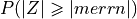$P(\vert Z\vert \geqslant \vert merrn\vert)$ , where $Z\sim\mathcal{N}(0,1/n)$
1. chi-square test for sum of squares of normalized error, sserrn: the test computes the p-value: $P(X \geqslant sserrn)$ , where $X\sim\chi^2_n$ (chi-square with n degrees of freedom);

A low p-value (e.g. below a significance level alpha=0.05) means that the model should be rejected (falsely rejected with probability alpha): the smaller the p-value, the more evidence there is to reject the model; each test computes:

the p-value pvalue
the result (success/failure): the boolean success=(pvalue > significance) which means that the model should be rejected when success=False with respect to the specified significance level

Parameters:

x (2D array of floats of shape (n, d)) – data points locations, with n the number of data points and d the space dimension (1, 2, or 3), each row of x is the coordinatates of one data point; note: for data in 1D (d=1), 1D array of shape (n,) is accepted for n data points
v (1D array of floats of shape (n,)) – data points values, with n the number of data points, v[i] is the data value at location x[i]
cov_model (CovModel1D or CovModel2D or CovModel3D) –
covariance model in 1D, 2D, or 3D, in same dimension as dimension of points (d), i.e.:
- CovModel1D for data in 1D (d=1)
- CovModel2D for data in 2D (d=2)
- CovModel3D for data in 3D (d=3)
or
- CovModel1D interpreted as an omni-directional covariance model whatever dimension of points (d);
v_err_std (1D array of floats of shape (n,), or float, default: 0.0) – standard deviation of error at data points, with n the number of data points; if v_err_std is a float, the same value is used for all data points; this means that at location x[i], the data value is considered as in a Gaussian distribution of mean v[i] and standard deviation v_err_std[i]
dmin (float, optional) – minimal distance between the data point to be estimated and the other ones, i.e. when estimating the value at x[i], all points x[j] at a distance less than dmin are not taking into account; note: this means that the cross-validation is no longer “leave-one-out” since more than one point may be ignored
mean_x (1D array-like of floats, or float, optional) –
kriging mean value at data points x
- if mean_x is a float, the same value is considered for any point;
- if mean_x=None (default): the mean of data values, i.e. mean of v, is considered for any point;
note: parameter mean_x is ignored if ordinary kriging is used as interpolator
var_x (1D array-like of floats, or float, optional) –
kriging variance value at data points x
- if var_x is a float, the same value is considered for any point
- if var_x=None (default): not used (use of covariance model only)
note: parameter var_x is ignored if ordinary kriging is used as interpolator
alpha_x (1D array-like of floats, or float, optional) –
azimuth angle in degrees at points x
- if alpha_x is a float, the same value is considered for any point
- if alpha_x=None (default): alpha_x=0.0 is used for any point
note: alpha_x is ignored if the covariance model is in 1D
beta_x (1D array-like of floats, or float, optional) –
dip angle in degrees at points x - if beta_x is a float, the same value is considered for any point - if beta_x=None (default): beta_x=0.0 is used for any point

note: beta_x is ignored if the covariance model is in 1D or 2D
gamma_x (1D array-like of floats, or float, optional) –
dip angle in degrees at points x
- if gamma_x is a float, the same value is considered for any point
- if gamma_x=None (default): gamma_x=0.0 is used for any point
note: gamma_x is ignored if the covariance model is in 1D or 2D
cov_model_non_stationarity_x_list (list, optional) –
list to set non-stationarities in covariance model; each entry must be a tuple (or list) cm_ns of length 2 or 3 with:
- cm_ns[0]: str: the name of the method of cov_model to be applied
- cm_ns[1]: 1D array-like of floats, or float: used to set the main parameter passed to the method:
  - if array-like: its size must be equal to nu, (the array is reshaped if needed), values at points x
  - if a float: same value at all points x
- cm_ns[2]: dict, optional: keyworkds arguments to be passed to the method
Examples (with the parameter arg is set from val)
- (‘multiply_w’, val) will apply cov_model.multiply_w(arg);
  this multipies the weight contribution of every elementary contribution of the covariance model
- (‘multiply_w’, val, {‘elem_ind’:0}) will apply cov_model.multiply_w(arg, elem_ind=0);
  this multipies the weight contribution of the elementary contribution of index 0 of the covariance model
- (‘multiply_r’, val) will apply cov_model.multiply_r(arg);
  this multipies the range in all direction of every elementary contribution of the covariance model
- (‘multiply_r’, val, {‘r_ind’:0}) will apply cov_model.multiply_r(arg, r_ind=0);
  this multipies the range in the first main direction (index 0) of every elementary contribution of the covariance model
- (‘multiply_r’, val, {‘r_ind’:0, ‘elem_ind’:0}) will apply cov_model.multiply_r(arg, r_ind=0, elem_ind=0);
  this multipies the range in the first main direction (index 0) of the elementary contribution of index 0 of the covariance model
significance (float, default: 0.05) – significance level for the two statisic tests, a float between 0 and 1, defining the success/failure of the two statistic tests (see above)
interpolator (function (callable), default: krige) – function used to do the interpolations
interpolator_kwargs (dict, optional) –
keyword arguments passed to interpolator; e.g. with interpolator=krige:
- interpolator_kwargs={‘method’:’ordinary_kriging’},
- interpolator_kwargs={‘method’:’simple_kriging’, ‘use_unique_neighborhood’:True}
print_result (bool, default: True) – indicates if the results (mean CRPS, and the 2 statistic tests) are printed, as well as some indicators
make_plot (bool, default: True) – indicates if a plot of the results is displayed (in a new “1x2” figure)
figsize (2-tuple, optional) – size of the new “1x2” figure (if make_plot=True)
nbins (int, optional) – number of bins in plotted histogram
logger (logging.Logger, optional) – logger (see package logging) if specified, messages are written via logger (no print)

Returns:

v_est (1D array of shape (n,)) – estimates at data points x by the interpolation
v_std (1D array of shape (n,)) – standard deviations at data points x by the interpolation
crps (1D array of shape (n,)) – CRPS of the prediction distribution (normal) at data points x
crps_def (float) – “default” crps, according to unbiased prediction with the standard deviation of the data values (see above)
pvalue (1D array of two floats) –
- pvalue[0]: p-value for the statistic test 1 (normal law test for mean of normalized error)
- pvalue[1]: p-value for the statistic test 2 (chi-square test for sum of squares of normalized error)
success (1D array of two bools) –
- success[i] = (pvalue[i] > significance), success (True) or failure (False) of the corresponding statistical test
if one False is obtained, it means that the model should be rejected

covModel.eval_at_points_1D(f, pts, nx, sx, ox, return_float_if_unique=True, logger=None)

Evaluates f at points - 1D.

Parameters:

f (function (callable), or array-like of floats, or float) –
function or value(s) in grid in input:
- if a function: function of 1 argument that returns a value for each location given by their coordinate in argument
- if array-like: its size must be equal to the number of grid cells (the array is reshaped if needed), values at grid cells; note the shape of the array is (nx,)
- if a float: same value at every grid cell
pts (2D array of floats of shape (n, 1)) – points at which the input fuction or value(s) has to be interpolated
nx (int) – number of grid cells along x axis
sx (float) – cell size along x axis
ox (float) –
origin of the grid along x axis (x coordinate of cell border)

Note: (ox, ) is the “bottom-lower-left” corner of the grid
return_float_if_unique (bool, default: True) – if True and if all output values are identical, then a float (the unique output value) is returned; otherwise: an array of shape (n,) is returned
logger (logging.Logger, optional) – logger (see package logging) if specified, messages are written via logger (no print)

Returns:

f_pts – array of output values at point pts of shape (n,); if return_float_if_unique=True and if all output values are identical, then a float (the unique output value) is returned

Return type:

array of floats, or float

covModel.eval_at_points_2D(f, pts, nx, ny, sx, sy, ox, oy, return_float_if_unique=True, logger=None)

Evaluates f at points - 2D.

Parameters:

f (function (callable), or array-like of floats, or float) –
function or value(s) in grid in input:
- if a function: function of 2 arguments that returns a value for each location given by their coordinates in argument
- if array-like: its size must be equal to the number of grid cells (the array is reshaped if needed), values at grid cells; note the shape of the array is (ny, nx)
- if a float: same value at every grid cell
pts (2D array of floats of shape (n, 2)) – points at which the input fuction or value(s) has to be interpolated
nx (int) – number of grid cells along x axis
ny (int) – number of grid cells along y axis
sx (float) – cell size along x axis
sy (float) – cell size along y axis
ox (float) – origin of the grid along x axis (x coordinate of cell border)
oy (float) –
origin of the grid along y axis (y coordinate of cell border)

Note: (ox, oy) is the “bottom-lower-left” corner of the grid
return_float_if_unique (bool, default: True) – if True and if all output values are identical, then a float (the unique output value) is returned; otherwise: an array of shape (n,) is returned
logger (logging.Logger, optional) – logger (see package logging) if specified, messages are written via logger (no print)

Returns:

f_pts – array of output values at point pts of shape (n,); if return_float_if_unique=True and if all output values are identical, then a float (the unique output value) is returned

Return type:

array of floats, or float

covModel.eval_at_points_3D(f, pts, nx, ny, nz, sx, sy, sz, ox, oy, oz, return_float_if_unique=True, logger=None)

Evaluates f at points - 3D.

Parameters:

f (function (callable), or array-like of floats, or float) –
function or value(s) in grid in input:
- if a function: function of 3 arguments that returns a value for each location given by their coordinates in argument
- if array-like: its size must be equal to the number of grid cells (the array is reshaped if needed), values at grid cells; note the shape of the array is (nz, ny, nx)
- if a float: same value at every grid cell
pts (2D array of floats of shape (n, 3)) – points at which the input fuction or value(s) has to be interpolated
nx (int) – number of grid cells along x axis
ny (int) – number of grid cells along y axis
nz (int) – number of grid cells along z axis
sx (float) – cell size along x axis
sy (float) – cell size along y axis
sz (float) – cell size along z axis
ox (float) – origin of the grid along x axis (x coordinate of cell border)
oy (float) – origin of the grid along y axis (y coordinate of cell border)
oz (float) –
origin of the grid along z axis (z coordinate of cell border)

Note: (ox, oy, oz) is the “bottom-lower-left” corner of the grid
return_float_if_unique (bool, default: True) – if True and if all output values are identical, then a float (the unique output value) is returned; otherwise: an array of shape (n,) is returned
logger (logging.Logger, optional) – logger (see package logging) if specified, messages are written via logger (no print)

Returns:

f_pts – array of output values at point pts of shape (n,); if return_float_if_unique=True and if all output values are identical, then a float (the unique output value) is returned

Return type:

array of floats, or float

covModel.eval_in_grid_1D(f, nx, sx, ox, return_float_if_unique=True, logger=None)

Evaluates f in grid - 1D.

Parameters:

f (function (callable), or array-like of floats, or float) –
function or value(s) in grid in input:
- if a function: function of 1 argument that returns a value for each location given by their coordinate in argument
- if array-like: its size must be equal to the number of grid cells (the array is reshaped if needed), values at grid cells; note the shape of the array is (nx,)
- if a float: same value at every grid cell
nx (int) – number of grid cells along x axis
sx (float) – cell size along x axis
ox (float) –
origin of the grid along x axis (x coordinate of cell border)

Note: (ox, ) is the “bottom-lower-left” corner of the grid
return_float_if_unique (bool, default: True) – if True and if all output values are identical, then a float (the unique output value) is returned; otherwise: an array of shape (nx,) is returned
logger (logging.Logger, optional) – logger (see package logging) if specified, messages are written via logger (no print)

Returns:

f_grid – array of output values in the grid (cell centers), of shape (nx,), f_grid[ix] is the value at the grid cell of index ix along x-axis; if return_float_if_unique=True and if all output values are identical, then a float (the unique output value) is returned

Return type:

array of floats, or float

covModel.eval_in_grid_2D(f, nx, ny, sx, sy, ox, oy, return_float_if_unique=True, logger=None)

Evaluates f in grid - 2D.

Parameters:

f (function (callable), or array-like of floats, or float) –
function or value(s) in grid in input:
- if a function: function of 2 arguments that returns a value for each location given by their coordinates in argument
- if array-like: its size must be equal to the number of grid cells (the array is reshaped if needed), values at grid cells; note the shape of the array is (ny, nx)
- if a float: same value at every grid cell
nx (int) – number of grid cells along x axis
ny (int) – number of grid cells along y axis
sx (float) – cell size along x axis
sy (float) – cell size along y axis
ox (float) – origin of the grid along x axis (x coordinate of cell border)
oy (float) –
origin of the grid along y axis (y coordinate of cell border)

Note: (ox, oy) is the “bottom-lower-left” corner of the grid
return_float_if_unique (bool, default: True) – if True and if all output values are identical, then a float (the unique output value) is returned; otherwise: an array of shape (ny, nx) is returned
logger (logging.Logger, optional) – logger (see package logging) if specified, messages are written via logger (no print)

Returns:

f_grid – array of output values in the grid (cell centers), of shape (ny, nx), f_grid[iy, ix] is the value at the grid cell of indices ix along x-axis, iy along y-axis; if return_float_if_unique=True and if all output values are identical, then a float (the unique output value) is returned

Return type:

array of floats, or float

covModel.eval_in_grid_3D(f, nx, ny, nz, sx, sy, sz, ox, oy, oz, return_float_if_unique=True, logger=None)

Evaluates f in grid - 3D.

Parameters:

f (function (callable), or array-like of floats, or float) –
function or value(s) in grid in input:
- if a function: function of 3 arguments that returns a value for each location given by their coordinates in argument
- if array-like: its size must be equal to the number of grid cells (the array is reshaped if needed), values at grid cells; note the shape of the array is (nz, ny, nx)
- if a float: same value at every grid cell
nx (int) – number of grid cells along x axis
ny (int) – number of grid cells along y axis
nz (int) – number of grid cells along z axis
sx (float) – cell size along x axis
sy (float) – cell size along y axis
sz (float) – cell size along z axis
ox (float) – origin of the grid along x axis (x coordinate of cell border)
oy (float) – origin of the grid along y axis (y coordinate of cell border)
oz (float) –
origin of the grid along z axis (z coordinate of cell border)

Note: (ox, oy, oz) is the “bottom-lower-left” corner of the grid
return_float_if_unique (bool, default: True) – if True and if all output values are identical, then a float (the unique output value) is returned; otherwise: an array of shape (nz, ny, nx) is returned
logger (logging.Logger, optional) – logger (see package logging) if specified, messages are written via logger (no print)

Returns:

f_grid – array of output values in the grid (cell centers), of shape (nz, ny, nx), f_grid[iz, iy, ix] is the value at the grid cell of indices ix along x-axis, iy along y-axis, iz along z-axis; if return_float_if_unique=True and if all output values are identical, then a float (the unique output value) is returned

Return type:

array of floats, or float

covModel.krige(x, v, xu, cov_model, v_err_std=0.0, method='ordinary_kriging', mean_x=None, mean_xu=None, var_x=None, var_xu=None, alpha_xu=None, beta_xu=None, gamma_xu=None, cov_model_non_stationarity_xu_list=None, use_unique_neighborhood=False, searchRadius=None, searchRadiusRelative=1.2, nneighborMax=12, pid=None, verbose=0, logger=None)

Interpolates data by kriging at given location(s).

This function performs kriging interpolation at locations xu of the values v measured at locations x.

Parameters:

x (2D array of floats of shape (n, d)) – data points locations, with n the number of data points and d the space dimension (1, 2, or 3), each row of x is the coordinatates of one data point; note: for data in 1D (d=1), 1D array of shape (n,) is accepted for n data points
v (1D array of floats of shape (n,)) – data points values, with n the number of data points, v[i] is the data value at location x[i]
xu (2D array of floats of shape (nu, d)) – points locations where the interpolation has to be done, with nu the number of points and d the space dimension (1, 2, or 3, same as for x), each row of xu is the coordinatates of one point; note: for data in 1D (d=1), 1D array of shape (nu,) is accepted for nu points
cov_model (CovModel1D or CovModel2D or CovModel3D) –
covariance model in 1D, 2D, or 3D, in same dimension as dimension of points (d), i.e.:
- CovModel1D for data in 1D (d=1)
- CovModel2D for data in 2D (d=2)
- CovModel3D for data in 3D (d=3)
or
- CovModel1D interpreted as an omni-directional covariance model whatever dimension of points (d);
note: the covariance model must be stationary, however, non stationarity is handled:
- local rotation by specifying alpha_xu (in 2D or 3D), beta_xu (in 3D), gamma_xu (in 3D)
- other non-stationarities by specifying cov_model_non_stationarity_xu_list (see below)
v_err_std (1D array of floats of shape (n,), or float, default: 0.0) – standard deviation of error at data points, with n the number of data points; if v_err_std is a float, the same value is used for all data points; this means that at location x[i], the data value is considered as in a Gaussian distribution of mean v[i] and standard deviation v_err_std[i]
method (str {'simple_kriging', 'ordinary_kriging'}, default: 'ordinary_kriging') – type of kriging; note: if method=’ordinary_kriging’, the parameters mean_x, mean_xu, var_x, var_xu are not used
mean_x (1D array-like of floats, or float, optional) –
kriging mean value at data points x
- if mean_x is a float, the same value is considered for any point
- if mean_x=None (default): the mean of data values, i.e. mean of v, is considered for any point
note: if method=ordinary_kriging, parameter mean_x is ignored
mean_xu (1D array-like of floats, or float, optional) –
kriging mean value at points xu
- if mean_xu is a float, the same value is considered for any point
- if mean_xu=None (default): the value mean_x (assumed to be a single float) is considered for any point
note: if method=ordinary_kriging, parameter mean_xu is ignored
var_x (1D array-like of floats, or float, optional) –
kriging variance value at data points x
- if var_x is a float, the same value is considered for any point
- if var_x=None (default): not used (use of covariance model only)
note: if method=ordinary_kriging, parameter var_x is ignored
var_xu (1D array-like of floats, or float, optional) –
kriging variance value at points xu
- if var_xu is a float, the same value is considered for any point
- if var_xu=None (default): not used (use of covariance model only)
note: if method=ordinary_kriging, parameter var_xu is ignored
alpha_xu (1D array-like of floats, or float, optional) –
azimuth angle in degrees at points xu
- if alpha_xu is a float, the same value is considered for any point
- if alpha_xu=None (default): alpha_xu=0.0 is used for any point
note: alpha_xu is ignored if the covariance model is in 1D
beta_xu (1D array-like of floats, or float, optional) –
dip angle in degrees at points xu
- if beta_xu is a float, the same value is considered for any point
- if beta_xu=None (default): beta_xu=0.0 is used for any point
note: beta_xu is ignored if the covariance model is in 1D or 2D
gamma_xu (1D array-like of floats, or float, optional) –
dip angle in degrees at points xu
- if gamma_xu is a float, the same value is considered for any point
- if gamma_xu=None (default): gamma_xu=0.0 is used for any point
note: gamma_xu is ignored if the covariance model is in 1D or 2D
cov_model_non_stationarity_xu_list (list, optional) –
list to set non-stationarities in covariance model; each entry must be a tuple (or list) cm_ns of length 2 or 3 with:
- cm_ns[0]: str: the name of the method of cov_model to be applied
- cm_ns[1]: 1D array-like of floats, or float: used to set the main parameter passed to the method:
  - if array-like: its size must be equal to nu, (the array is reshaped if needed), values at points xu
  - if a float: same value at all points xu
- cm_ns[2]: dict, optional: keyworkds arguments to be passed to the method
Examples (with the parameter arg is set from val)
- (‘multiply_w’, val) will apply cov_model.multiply_w(arg);
  this multipies the weight contribution of every elementary contribution of the covariance model
- (‘multiply_w’, val, {‘elem_ind’:0}) will apply cov_model.multiply_w(arg, elem_ind=0);
  this multipies the weight contribution of the elementary contribution of index 0 of the covariance model
- (‘multiply_r’, val) will apply cov_model.multiply_r(arg);
  this multipies the range in all direction of every elementary contribution of the covariance model
- (‘multiply_r’, val, {‘r_ind’:0}) will apply cov_model.multiply_r(arg, r_ind=0);
  this multipies the range in the first main direction (index 0) of every elementary contribution of the covariance model
- (‘multiply_r’, val, {‘r_ind’:0, ‘elem_ind’:0}) will apply cov_model.multiply_r(arg, r_ind=0, elem_ind=0);
  this multipies the range in the first main direction (index 0) of the elementary contribution of index 0 of the covariance model
use_unique_neighborhood (bool, default: False) –
indicates if a unique neighborhood is used:
- if True: all data points are taken into account, and the kriging matrix is computed once; the parameters searchRadius, searchRadiusRelative, nneighborMax are not used, and alpha_xu, beta_xu, gamma_xu must be None or constant and any non-stationarity set in cov_model_non_stationarity_xu_list must be constant (i.e. cm_ns[1] must be constant for each entry cm_ns in cov_model_non_stationarity_xu_list)
- if False: only data points within a search neighborhood (ellipsoid) are taken into account according to searchRadius, searchRadiusRelative, nneighborMax
searchRadius (float, optional) – if specified, i.e. not None: radius of the search neighborhood (ellipsoid with same radii along each axis), i.e. the data points at distance to the estimated point greater than searchRadius are not taken into account in the kriging system; if searchRadius is not None, then searchRadiusRelative is not used; by default (searchRadius=None): searchRadiusRelative is used to define the search ellipsoid;
searchRadiusRelative (float, default: 1.2) – used only if searchRadius is None; indicates how the search ellipsoid is limited (should be positive): let r_i be the ranges of the covariance model along its main axes, when estimating/simulating a cell x, a cell y is taken into account iff it is within the ellipsoid centered at x of half axes equal to searchRadiusRelative * r_i; (note that the distances to the central node are computed in the axes sytem supporting the covariance model and accounting for anisotropy given by the ranges)
nneighborMax (int, default: 12) – maximal number of neighbors (data points) taken into account in the kriging system; the data points the closest to the estimated points are taken into account; note: if nneighborMax=None or nneighborMax<0, then nneighborMax is set to the number of data points
pid (int, optional) – process id of the caller (used with multiprocessing)
verbose (int, default: 0) – verbose mode, higher implies more printing (info)
logger (logging.Logger, optional) – logger (see package logging) if specified, messages are written via logger (no print)

Returns:

vu (1D array of shape (nu,)) – kriging estimates at points xu; note: vu[j]=numpy.nan if there is no data point in the neighborhood of xu[j] (see parameters searchRadius, searchRadiusRelative, nneighborMax)
vu_std (1D array of shape (nu,)) – kriging standard deviations at points xu; note: vu_std[j]=numpy.nan if there is no data point in the neighborhood of xu[j] (see parameters searchRadius, searchRadiusRelative, nneighborMax)

covModel.plot_variogramCloud1D(h, g, decim=1.0, seed=None, show_xlabel=True, show_ylabel=True, grid=True, **kwargs)

Plots a variogram cloud (1D) (in the current figure axis).

Parameters:

h (1D array of floats) – see g
g (1D array of floats) – h and g (of same length) are the coordinates of the points (lag values and gamma values resp.) in the variogram cloud
decim (float, default: 1.0) – the variogram cloud plotted after decimation by taking into account a proportion of decim points, randomly chosen; by default (1): all points are plotted
seed (int, optional) – seed number used to initialize the random number generator (used if decim<1)
show_xlabel (bool, default: True) – indicates if (default) label for abscissa is displayed
show_ylabel (bool, default: True) – indicates if (default) label for ordinate is displayed
grid (bool, default: True) – indicates if a grid is plotted
kwargs (dict) – keyword arguments passed to the funtion matplotlib.pyplot.plot

covModel.plot_variogramExp1D(hexp, gexp, cexp, show_count=True, show_ylabel=True, show_xlabel=True, grid=True, **kwargs)

Plots an experimental variogram (1D) (in the current figure axis).

Parameters:

hexp (1D array of floats) – see gexp
gexp (1D array of floats) – hexp and gexp (of same length) are the coordinates of the points (lag values and gamma values resp.) in the experimental variogram
cexp (1D array of ints) – array of same length as hexp, gexp, counters, number of points (pairs of data points considered) comming from the variogram cloud that defines each point in the experimental variogram
show_count (bool, default: True) – indicates if counters (cexp) are displayed on the plot
show_xlabel (bool, default: True) – indicates if (default) label for abscissa is displayed
show_ylabel (bool, default: True) – indicates if (default) label for ordinate is displayed
grid (bool, default: True) – indicates if a grid is plotted
kwargs (dict) – keyword arguments passed to the funtion matplotlib.pyplot.plot

covModel.rotationMatrix2D(alpha=0.0)

Returns the 2x2 matrix of rotation defining axes of covariance model in 2D.

The function returns the 2x2 matrix m for changing the coordinates system from Ox’y’ to Oxy, where the system Ox’y’ is obtained from the system Oxy by applying a rotation of angle -alpha,

$m = \left(\begin{array}{cc} \cos\alpha & \sin\alpha\\ -\sin\alpha & \cos\alpha \end{array}\right)$

i.e. the columns of m are the new axes expressed in the system Oxy.

Parameters:: alpha (float, default: 0.0) – azimuth angle in degrees
Returns:: mrot – rotation matrix (see above)
Return type:: 2D array of shape (2, 2)

covModel.rotationMatrix3D(alpha=0.0, beta=0.0, gamma=0.0)

Returns the 3x3 matrix of rotation defining axes of covariance model in 3D.

The function returns the 3x3 matrix m for changing the coordinates system from Ox’’’y’’’z’’’ to Oxyz, where the system Ox’’’y’’’’z’’’ is obtained from the system Oxyz as follows:

# Oxyz      -- rotation of angle -alpha around Oz  --> Ox'y'z'
# Ox'y'z'   -- rotation of angle -beta  around Ox' --> Ox''y''z''
# Ox''y''z''-- rotation of angle -gamma around Oy''--> Ox'''y'''z'''

The matrix m is given by

$m = \left(\begin{array}{rrr} \cos\alpha \cdot \cos\gamma + \sin\alpha \cdot \sin\beta \cdot \sin\gamma & \sin\alpha \cdot \cos\beta & - \cos\alpha \cdot \sin\gamma + \sin\alpha \cdot \sin\beta \cdot \cos\gamma \\ - \sin\alpha \cdot \cos\gamma + \cos\alpha \cdot \sin\beta \cdot \sin\gamma & \cos\alpha \cdot \cos\beta & \sin\alpha \cdot \sin\gamma + \cos\alpha \cdot \sin\beta \cdot \cos\gamma \\ \cos\beta \cdot \sin\gamma & - \sin\beta & \cos\beta \cdot \cos\gamma \end{array}\right)$

i.e. the columns of m are the new axes expressed in the system Oxyz.

Parameters:

alpha (float, default: 0.0) – azimuth angle in degrees
beta (float, default: 0.0) – dip angle in degrees
plunge (float, default: 0.0) – azimuth angle in degrees

Returns:

mrot – rotation matrix (see above)

Return type:

2D array of shape (3, 3)

covModel.sgs(x, v, xu, cov_model, v_err_std=0.0, method='ordinary_kriging', mean_x=None, mean_xu=None, var_x=None, var_xu=None, alpha_xu=None, beta_xu=None, gamma_xu=None, cov_model_non_stationarity_xu_list=None, searchRadius=None, searchRadiusRelative=1.2, nneighborMax=12, nreal=1, seed=None, pid=None, verbose=0, logger=None)

Performs Sequential Gaussian Simulation (SGS) at given location(s).

This function does SGS at locations xu, given data points locations x with values v.

Parameters:

x (2D array of floats of shape (n, d)) – data points locations, with n the number of data points and d the space dimension (1, 2, or 3), each row of x is the coordinatates of one data point; note: for data in 1D (d=1), 1D array of shape (n,) is accepted for n data points
v (1D array of floats of shape (n,)) – data points values, with n the number of data points, v[i] is the data value at location x[i]
xu (2D array of floats of shape (nu, d)) – points locations where the interpolation has to be done, with nu the number of points and d the space dimension (1, 2, or 3, same as for x), each row of xu is the coordinatates of one point; note: for data in 1D (d=1), 1D array of shape (nu,) is accepted for nu points
cov_model (CovModel1D or CovModel2D or CovModel3D) –
covariance model in 1D, 2D, or 3D, in same dimension as dimension of points (d), i.e.:
- CovModel1D for data in 1D (d=1)
- CovModel2D for data in 2D (d=2)
- CovModel3D for data in 3D (d=3)
or
- CovModel1D interpreted as an omni-directional covariance model whatever dimension of points (d);
note: the covariance model must be stationary, however, non stationarity is handled:
- local rotation by specifying alpha_xu (in 2D or 3D), beta_xu (in 3D), gamma_xu (in 3D)
- other non-stationarities by specifying cov_model_non_stationarity_xu_list (see below)
v_err_std (1D array of floats of shape (n,), or float, default: 0.0) – standard deviation of error at data points, with n the number of data points; if v_err_std is a float, the same value is used for all data points; this means that at location x[i], the data value is considered as in a Gaussian distribution of mean v[i] and standard deviation v_err_std[i]
method (str {'simple_kriging', 'ordinary_kriging'}, default: 'ordinary_kriging') – type of kriging; note: if method=’ordinary_kriging’, the parameters mean_x, mean_xu, var_x, var_xu are not used
mean_x (1D array-like of floats, or float, optional) –
kriging mean value at data points x
- if mean_x is a float, the same value is considered for any point
- if mean_x=None (default): the mean of data values, i.e. mean of v, is considered for any point
note: if method=ordinary_kriging, parameter mean_x is ignored
mean_xu (1D array-like of floats, or float, optional) –
kriging mean value at points xu
- if mean_xu is a float, the same value is considered for any point
- if mean_xu=None (default): the value mean_x (assumed to be a single float) is considered for any point
note: if method=ordinary_kriging, parameter mean_xu is ignored
var_x (1D array-like of floats, or float, optional) –
kriging variance value at data points x
- if var_x is a float, the same value is considered for any point
- if var_x=None (default): not used (use of covariance model only)
note: if method=ordinary_kriging, parameter var_x is ignored
var_xu (1D array-like of floats, or float, optional) –
kriging variance value at points xu
- if var_xu is a float, the same value is considered for any point
- if var_xu=None (default): not used (use of covariance model only)
note: if method=ordinary_kriging, parameter var_xu is ignored
alpha_xu (1D array-like of floats, or float, optional) –
azimuth angle in degrees at points xu
- if alpha_xu is a float, the same value is considered for any point
- if alpha_xu=None (default): alpha_xu=0.0 is used for any point
note: alpha_xu is ignored if the covariance model is in 1D
beta_xu (1D array-like of floats, or float, optional) –
dip angle in degrees at points xu
- if beta_xu is a float, the same value is considered for any point
- if beta_xu=None (default): beta_xu=0.0 is used for any point
note: beta_xu is ignored if the covariance model is in 1D or 2D
gamma_xu (1D array-like of floats, or float, optional) –
dip angle in degrees at points xu
- if gamma_xu is a float, the same value is considered for any point
- if gamma_xu=None (default): gamma_xu=0.0 is used for any point
note: gamma_xu is ignored if the covariance model is in 1D or 2D
cov_model_non_stationarity_xu_list (list, optional) –
list to set non-stationarities in covariance model; each entry must be a tuple (or list) cm_ns of length 2 or 3 with:
- cm_ns[0]: str: the name of the method of cov_model to be applied
- cm_ns[1]: 1D array-like of floats, or float: used to set the main parameter passed to the method:
  - if array-like: its size must be equal to nu, (the array is reshaped if needed), values at points xu
  - if a float: same value at all points xu
- cm_ns[2]: dict, optional: keyworkds arguments to be passed to the method
Examples (with the parameter arg is set from val)
- (‘multiply_w’, val) will apply cov_model.multiply_w(arg);
  this multipies the weight contribution of every elementary contribution of the covariance model
- (‘multiply_w’, val, {‘elem_ind’:0}) will apply cov_model.multiply_w(arg, elem_ind=0);
  this multipies the weight contribution of the elementary contribution of index 0 of the covariance model
- (‘multiply_r’, val) will apply cov_model.multiply_r(arg);
  this multipies the range in all direction of every elementary contribution of the covariance model
- (‘multiply_r’, val, {‘r_ind’:0}) will apply cov_model.multiply_r(arg, r_ind=0);
  this multipies the range in the first main direction (index 0) of every elementary contribution of the covariance model
- (‘multiply_r’, val, {‘r_ind’:0, ‘elem_ind’:0}) will apply cov_model.multiply_r(arg, r_ind=0, elem_ind=0);
  this multipies the range in the first main direction (index 0) of the elementary contribution of index 0 of the covariance model
searchRadius (float, optional) – if specified, i.e. not None: radius of the search neighborhood (ellipsoid with same radii along each axis), i.e. the data points at distance to the estimated point greater than searchRadius are not taken into account in the kriging system; if searchRadius is not None, then searchRadiusRelative is not used; by default (searchRadius=None): searchRadiusRelative is used to define the search ellipsoid;
searchRadiusRelative (float, default: 1.2) – used only if searchRadius is None; indicates how the search ellipsoid is limited (should be positive): let r_i be the ranges of the covariance model along its main axes, when estimating/simulating a cell x, a cell y is taken into account iff it is within the ellipsoid centered at x of half axes equal to searchRadiusRelative * r_i; (note that the distances to the central node are computed in the axes sytem supporting the covariance model and accounting for anisotropy given by the ranges)
nneighborMax (int, default: 12) – maximal number of neighbors (data points) taken into account in the kriging system; the data points the closest to the estimated points are taken into account
nreal (int, default: 1) – number of realization(s)
seed (int, optional) – seed for initializing random number generator
pid (int, optional) – process id of the caller (used with multiprocessing)
verbose (int, default: 0) – verbose mode, higher implies more printing (info)
logger (logging.Logger, optional) – logger (see package logging) if specified, messages are written via logger (no print)

Returns:

vu – simulated values at points xu - vu[i, j] value of the i-th realization at point xu[j]

Return type:

2D array of shape (nreal, nu)

covModel.sgs_at_inequality_data_points(x, v, x_ineq, cov_model, v_err_std=0.0, v_ineq_min=None, v_ineq_max=None, method='ordinary_kriging', mean_x=None, mean_x_ineq=None, var_x=None, var_x_ineq=None, alpha_x_ineq=None, beta_x_ineq=None, gamma_x_ineq=None, cov_model_non_stationarity_x_ineq_list=None, searchRadius=None, searchRadiusRelative=1.2, nneighborMax=12, nGibbsSamplerPath=50, nreal=1, seed=None, pid=None, verbose=0, logger=None)

Performs Sequential Gaussian Simulation (SGS) at inequality data point(s).

This function does SGS at locations x_ineq, given data points locations x with values v.

Parameters:

x (2D array of floats of shape (n, d)) – data points locations, with n the number of data points and d the space dimension (1, 2, or 3), each row of x is the coordinatates of one data point; note: for data in 1D (d=1), 1D array of shape (n,) is accepted for n data points
v (1D array of floats of shape (n,)) – data points values, with n the number of data points, v[i] is the data value at location x[i]
x_ineq (2D array of floats of shape (n_ineq, d)) – points locations where the interpolation has to be done, with n_ineq the number of points and d the space dimension (1, 2, or 3, same as for x), each row of x_ineq is the coordinatates of one point; note: for data in 1D (d=1), 1D array of shape (n_ineq,) is accepted for n_ineq points
cov_model (CovModel1D or CovModel2D or CovModel3D) –
covariance model in 1D, 2D, or 3D, in same dimension as dimension of points (d), i.e.:
- CovModel1D for data in 1D (d=1)
- CovModel2D for data in 2D (d=2)
- CovModel3D for data in 3D (d=3)
or
- CovModel1D interpreted as an omni-directional covariance model whatever dimension of points (d);
note: the covariance model must be stationary, however, non stationarity is handled:
- local rotation by specifying alpha_x_ineq (in 2D or 3D), beta_x_ineq (in 3D), gamma_x_ineq (in 3D)
- other non-stationarities by specifying cov_model_non_stationarity_x_ineq_list (see below)
v_err_std (1D array of floats of shape (n,), or float, default: 0.0) – standard deviation of error at data points, with n the number of data points; if v_err_std is a float, the same value is used for all data points; this means that at location x[i], the data value is considered as in a Gaussian distribution of mean v[i] and standard deviation v_err_std[i]
v_ineq_min (1D array of floats of shape (n_ineq,), or float, optional) – minimal value (lower bound) for inequality data points, with n_ineq the number of inequality data points (v_ineq_min[i] is the value for the location x_ineq[i]); if v_ineq_min is a float, the same value is used for all inequality data points; if v_ineq_min=None (default), no minimal value is considered for any inequality data point; note: v_ineq_min[i] set to np.nan or -np.inf means that there is no minimal value for point x_ineq[i]
v_ineq_max (1D array of floats of shape (n_ineq,), or float, optional) – maximal value (upper bound) for inequality data points, with n_ineq the number of inequality data points (v_ineq_max[i] is the value for the location x_ineq[i]); if v_ineq_max is a float, the same value is used for all inequality data points; if v_ineq_max=None (default), no maximal value is considered for any inequality data point; note: v_ineq_max[i] set to np.nan or np.inf means that there is no maximal value for point x_ineq[i]
method (str {'simple_kriging', 'ordinary_kriging'}, default: 'ordinary_kriging') – type of kriging; note: if method=’ordinary_kriging’, the parameters mean_x, mean_x_ineq, var_x, var_x_ineq are not used
mean_x (1D array-like of floats, or float, optional) –
kriging mean value at data points x
- if mean_x is a float, the same value is considered for any point
- if mean_x=None (default): the mean of data values, i.e. mean of v, is considered for any point
note: if method=ordinary_kriging, parameter mean_x is ignored
mean_x_ineq (1D array-like of floats, or float, optional) –
kriging mean value at points x_ineq
- if mean_x_ineq is a float, the same value is considered for any point
- if mean_x_ineq=None (default): the value mean_x (assumed to be a single float) is considered for any point
note: if method=ordinary_kriging, parameter mean_x_ineq is ignored
var_x (1D array-like of floats, or float, optional) –
kriging variance value at data points x
- if var_x is a float, the same value is considered for any point
- if var_x=None (default): not used (use of covariance model only)
note: if method=ordinary_kriging, parameter var_x is ignored
var_x_ineq (1D array-like of floats, or float, optional) –
kriging variance value at points x_ineq
- if var_x_ineq is a float, the same value is considered for any point
- if var_x_ineq=None (default): not used (use of covariance model only)
note: if method=ordinary_kriging, parameter var_x_ineq is ignored
alpha_x_ineq (1D array-like of floats, or float, optional) –
azimuth angle in degrees at points x_ineq
- if alpha_x_ineq is a float, the same value is considered for any point
- if alpha_x_ineq=None (default): alpha_x_ineq=0.0 is used for any point
note: alpha_x_ineq is ignored if the covariance model is in 1D
beta_x_ineq (1D array-like of floats, or float, optional) –
dip angle in degrees at points x_ineq
- if beta_x_ineq is a float, the same value is considered for any point
- if beta_x_ineq=None (default): beta_x_ineq=0.0 is used for any point
note: beta_x_ineq is ignored if the covariance model is in 1D or 2D
gamma_x_ineq (1D array-like of floats, or float, optional) –
dip angle in degrees at points x_ineq
- if gamma_x_ineq is a float, the same value is considered for any point
- if gamma_x_ineq=None (default): gamma_x_ineq=0.0 is used for any point
note: gamma_x_ineq is ignored if the covariance model is in 1D or 2D
cov_model_non_stationarity_x_ineq_list (list, optional) –
list to set non-stationarities in covariance model; each entry must be a tuple (or list) cm_ns of length 2 or 3 with:
- cm_ns[0]: str: the name of the method of cov_model to be applied
- cm_ns[1]: 1D array-like of floats, or float: used to set the main parameter passed to the method:
  - if array-like: its size must be equal to n_ineq, (the array is reshaped if needed), values at points x_ineq
  - if a float: same value at all points x_ineq
- cm_ns[2]: dict, optional: keyworkds arguments to be passed to the method
Examples (with the parameter arg is set from val)
- (‘multiply_w’, val) will apply cov_model.multiply_w(arg);
  this multipies the weight contribution of every elementary contribution of the covariance model
- (‘multiply_w’, val, {‘elem_ind’:0}) will apply cov_model.multiply_w(arg, elem_ind=0);
  this multipies the weight contribution of the elementary contribution of index 0 of the covariance model
- (‘multiply_r’, val) will apply cov_model.multiply_r(arg);
  this multipies the range in all direction of every elementary contribution of the covariance model
- (‘multiply_r’, val, {‘r_ind’:0}) will apply cov_model.multiply_r(arg, r_ind=0);
  this multipies the range in the first main direction (index 0) of every elementary contribution of the covariance model
- (‘multiply_r’, val, {‘r_ind’:0, ‘elem_ind’:0}) will apply cov_model.multiply_r(arg, r_ind=0, elem_ind=0);
  this multipies the range in the first main direction (index 0) of the elementary contribution of index 0 of the covariance model
searchRadius (float, optional) – if specified, i.e. not None: radius of the search neighborhood (ellipsoid with same radii along each axis), i.e. the data points at distance to the estimated point greater than searchRadius are not taken into account in the kriging system; if searchRadius is not None, then searchRadiusRelative is not used; by default (searchRadius=None): searchRadiusRelative is used to define the search ellipsoid;
searchRadiusRelative (float, default: 1.2) – used only if searchRadius is None; indicates how the search ellipsoid is limited (should be positive): let r_i be the ranges of the covariance model along its main axes, when estimating/simulating a cell x, a cell y is taken into account iff it is within the ellipsoid centered at x of half axes equal to searchRadiusRelative * r_i; (note that the distances to the central node are computed in the axes sytem supporting the covariance model and accounting for anisotropy given by the ranges)
nneighborMax (int, default: 12) – maximal number of neighbors (data points) taken into account in the kriging system; the data points the closest to the estimated points are taken into account
nGibbsSamplerPath (int, default: 50) – number of Gibbs sampler paths for simulating values at inequality data points
nreal (int, default: 1) – number of realization(s)
seed (int, optional) – seed for initializing random number generator
pid (int, optional) – process id of the caller (used with multiprocessing)
verbose (int, default: 0) – verbose mode, higher implies more printing (info)
logger (logging.Logger, optional) – logger (see package logging) if specified, messages are written via logger (no print)

Returns:

v_ineq – simulated values at points x_ineq - v_ineq[i, j] value of the i-th realization at point x_ineq[j]

Return type:

2D array of shape (nreal, n_ineq)

covModel.sgs_at_inequality_data_points_mp(x, v, x_ineq, cov_model, v_err_std=0.0, v_ineq_min=None, v_ineq_max=None, method='ordinary_kriging', mean_x=None, mean_x_ineq=None, var_x=None, var_x_ineq=None, alpha_x_ineq=None, beta_x_ineq=None, gamma_x_ineq=None, cov_model_non_stationarity_x_ineq_list=None, searchRadius=None, searchRadiusRelative=1.2, nneighborMax=12, nGibbsSamplerPath=50, nreal=1, seed=None, verbose=0, nproc=-1, logger=None)

Computes the same as the function sgs_at_inequality_data_points(), using multiprocessing.

All the parameters except nproc are the same as those of the function sgs_at_inequality_data_points().

This function launches parallel processes [parallel calls of the function sgs_at_inequality_data_points()]; the set of realizations (specified by nreal) is distributed in a balanced way over the processes.

The number of processes used (in parallel) is determined by the parameter nproc (int, default: -1); a negative number (or zero), -n <= 0, can be specified to use the total number of cpu(s) of the system except n; nproc is finally at maximum equal to nreal but at least 1 by applying:

if nproc >= 1, then nproc = max(min(nproc, nreal), 1) is used
if nproc = -n <= 0, then nproc = max(min(nmax-n, nreal), 1) is used, where nmax is the total number of cpu(s) of the system (retrieved by multiprocessing.cpu_count())

Note: if nproc=None, nproc=-1 is used.

Note: specifying a seed guarantees reproducible results whatever the number of processes used.

See function sgs_at_inequality_data_points() for details.

covModel.sgs_at_inequality_data_points_seq(x, v, x_ineq, cov_model, v_err_std=0.0, v_ineq_min=None, v_ineq_max=None, method='ordinary_kriging', mean_x=None, mean_x_ineq=None, var_x=None, var_x_ineq=None, alpha_x_ineq=None, beta_x_ineq=None, gamma_x_ineq=None, cov_model_non_stationarity_x_ineq_list=None, searchRadius=None, searchRadiusRelative=1.2, nneighborMax=12, nGibbsSamplerPath_burn_in=50, nGibbsSamplerPath_intermediate=10, nreal=1, seed=None, verbose=0, logger=None)

Performs Sequential Gaussian Simulation (SGS) at inequality data point(s).

This function does SGS at locations x_ineq, given data points locations x with values v.

A sequence of realizations is done, via a Gibbs sampler in a unique Markov chain Monte Carlo: the first realization is taken after a “burn-in period”, then each next realization are taken after every “intermediate period”. Note that the all the realizations depend on the same seed number or intialization of the random number generator.

Parameters:

x (2D array of floats of shape (n, d)) – data points locations, with n the number of data points and d the space dimension (1, 2, or 3), each row of x is the coordinatates of one data point; note: for data in 1D (d=1), 1D array of shape (n,) is accepted for n data points
v (1D array of floats of shape (n,)) – data points values, with n the number of data points, v[i] is the data value at location x[i]
x_ineq (2D array of floats of shape (n_ineq, d)) – points locations where the interpolation has to be done, with n_ineq the number of points and d the space dimension (1, 2, or 3, same as for x), each row of x_ineq is the coordinatates of one point; note: for data in 1D (d=1), 1D array of shape (n_ineq,) is accepted for n_ineq points
cov_model (CovModel1D or CovModel2D or CovModel3D) –
covariance model in 1D, 2D, or 3D, in same dimension as dimension of points (d), i.e.:
- CovModel1D for data in 1D (d=1)
- CovModel2D for data in 2D (d=2)
- CovModel3D for data in 3D (d=3)
or
- CovModel1D interpreted as an omni-directional covariance model whatever dimension of points (d);
note: the covariance model must be stationary, however, non stationarity is handled:
- local rotation by specifying alpha_x_ineq (in 2D or 3D), beta_x_ineq (in 3D), gamma_x_ineq (in 3D)
- other non-stationarities by specifying cov_model_non_stationarity_x_ineq_list (see below)
v_err_std (1D array of floats of shape (n,), or float, default: 0.0) – standard deviation of error at data points, with n the number of data points; if v_err_std is a float, the same value is used for all data points; this means that at location x[i], the data value is considered as in a Gaussian distribution of mean v[i] and standard deviation v_err_std[i]
v_ineq_min (1D array of floats of shape (n_ineq,), or float, optional) – minimal value (lower bound) for inequality data points, with n_ineq the number of inequality data points (v_ineq_min[i] is the value for the location x_ineq[i]); if v_ineq_min is a float, the same value is used for all inequality data points; if v_ineq_min=None (default), no minimal value is considered for any inequality data point; note: v_ineq_min[i] set to np.nan or -np.inf means that there is no minimal value for point x_ineq[i]
v_ineq_max (1D array of floats of shape (n_ineq,), or float, optional) – maximal value (upper bound) for inequality data points, with n_ineq the number of inequality data points (v_ineq_max[i] is the value for the location x_ineq[i]); if v_ineq_max is a float, the same value is used for all inequality data points; if v_ineq_max=None (default), no maximal value is considered for any inequality data point; note: v_ineq_max[i] set to np.nan or np.inf means that there is no maximal value for point x_ineq[i]
method (str {'simple_kriging', 'ordinary_kriging'}, default: 'ordinary_kriging') – type of kriging; note: if method=’ordinary_kriging’, the parameters mean_x, mean_x_ineq, var_x, var_x_ineq are not used
mean_x (1D array-like of floats, or float, optional) –
kriging mean value at data points x
- if mean_x is a float, the same value is considered for any point
- if mean_x=None (default): the mean of data values, i.e. mean of v, is considered for any point
note: if method=ordinary_kriging, parameter mean_x is ignored
mean_x_ineq (1D array-like of floats, or float, optional) –
kriging mean value at points x_ineq
- if mean_x_ineq is a float, the same value is considered for any point
- if mean_x_ineq=None (default): the value mean_x (assumed to be a single float) is considered for any point
note: if method=ordinary_kriging, parameter mean_x_ineq is ignored
var_x (1D array-like of floats, or float, optional) –
kriging variance value at data points x
- if var_x is a float, the same value is considered for any point
- if var_x=None (default): not used (use of covariance model only)
note: if method=ordinary_kriging, parameter var_x is ignored
var_x_ineq (1D array-like of floats, or float, optional) –
kriging variance value at points x_ineq
- if var_x_ineq is a float, the same value is considered for any point
- if var_x_ineq=None (default): not used (use of covariance model only)
note: if method=ordinary_kriging, parameter var_x_ineq is ignored
alpha_x_ineq (1D array-like of floats, or float, optional) –
azimuth angle in degrees at points x_ineq
- if alpha_x_ineq is a float, the same value is considered for any point
- if alpha_x_ineq=None (default): alpha_x_ineq=0.0 is used for any point
note: alpha_x_ineq is ignored if the covariance model is in 1D
beta_x_ineq (1D array-like of floats, or float, optional) –
dip angle in degrees at points x_ineq
- if beta_x_ineq is a float, the same value is considered for any point
- if beta_x_ineq=None (default): beta_x_ineq=0.0 is used for any point
note: beta_x_ineq is ignored if the covariance model is in 1D or 2D
gamma_x_ineq (1D array-like of floats, or float, optional) –
dip angle in degrees at points x_ineq
- if gamma_x_ineq is a float, the same value is considered for any point
- if gamma_x_ineq=None (default): gamma_x_ineq=0.0 is used for any point
note: gamma_x_ineq is ignored if the covariance model is in 1D or 2D
cov_model_non_stationarity_x_ineq_list (list, optional) –
list to set non-stationarities in covariance model; each entry must be a tuple (or list) cm_ns of length 2 or 3 with:
- cm_ns[0]: str: the name of the method of cov_model to be applied
- cm_ns[1]: 1D array-like of floats, or float: used to set the main parameter passed to the method:
  - if array-like: its size must be equal to n_ineq, (the array is reshaped if needed), values at points x_ineq
  - if a float: same value at all points x_ineq
- cm_ns[2]: dict, optional: keyworkds arguments to be passed to the method
Examples (with the parameter arg is set from val)
- (‘multiply_w’, val) will apply cov_model.multiply_w(arg);
  this multipies the weight contribution of every elementary contribution of the covariance model
- (‘multiply_w’, val, {‘elem_ind’:0}) will apply cov_model.multiply_w(arg, elem_ind=0);
  this multipies the weight contribution of the elementary contribution of index 0 of the covariance model
- (‘multiply_r’, val) will apply cov_model.multiply_r(arg);
  this multipies the range in all direction of every elementary contribution of the covariance model
- (‘multiply_r’, val, {‘r_ind’:0}) will apply cov_model.multiply_r(arg, r_ind=0);
  this multipies the range in the first main direction (index 0) of every elementary contribution of the covariance model
- (‘multiply_r’, val, {‘r_ind’:0, ‘elem_ind’:0}) will apply cov_model.multiply_r(arg, r_ind=0, elem_ind=0);
  this multipies the range in the first main direction (index 0) of the elementary contribution of index 0 of the covariance model
searchRadius (float, optional) – if specified, i.e. not None: radius of the search neighborhood (ellipsoid with same radii along each axis), i.e. the data points at distance to the estimated point greater than searchRadius are not taken into account in the kriging system; if searchRadius is not None, then searchRadiusRelative is not used; by default (searchRadius=None): searchRadiusRelative is used to define the search ellipsoid;
searchRadiusRelative (float, default: 1.2) – used only if searchRadius is None; indicates how the search ellipsoid is limited (should be positive): let r_i be the ranges of the covariance model along its main axes, when estimating/simulating a cell x, a cell y is taken into account iff it is within the ellipsoid centered at x of half axes equal to searchRadiusRelative * r_i; (note that the distances to the central node are computed in the axes sytem supporting the covariance model and accounting for anisotropy given by the ranges)
nneighborMax (int, default: 12) – maximal number of neighbors (data points) taken into account in the kriging system; the data points the closest to the estimated points are taken into account
nGibbsSamplerPath_burn_in (int, default: 50) – burn-in period (number of Gibbs sampler paths, >= 1) of the McMC (for simulating values at inequality data points, for the first realization)
nGibbsSamplerPath_intermediate (int, default: 10) – intermediate period (number of Gibbs sampler paths, >= 1) of the McMC (for simulating values at inequality data points, for realization from the 2nd one)
nreal (int, default: 1) – number of realization(s)
seed (int, optional) – seed for initializing random number generator
verbose (int, default: 0) – verbose mode, higher implies more printing (info)
logger (logging.Logger, optional) – logger (see package logging) if specified, messages are written via logger (no print)

Returns:

v_ineq – simulated values at points x_ineq - v_ineq[i, j] value of the i-th realization at point x_ineq[j]

Return type:

2D array of shape (nreal, n_ineq)

covModel.sgs_at_inequality_data_points_slow(x, v, x_ineq, cov_model, v_err_std=0.0, v_ineq_min=None, v_ineq_max=None, method='ordinary_kriging', mean_x=None, mean_x_ineq=None, var_x=None, var_x_ineq=None, alpha_x_ineq=None, beta_x_ineq=None, gamma_x_ineq=None, cov_model_non_stationarity_x_ineq_list=None, searchRadius=None, searchRadiusRelative=1.2, nneighborMax=12, nGibbsSamplerPath=50, nreal=1, seed=None, pid=None, verbose=0, logger=None)

Performs Sequential Gaussian Simulation (SGS) at inequality data point(s).

This function does SGS at locations x_ineq, given data points locations x with values v.

Parameters:

x (2D array of floats of shape (n, d)) – data points locations, with n the number of data points and d the space dimension (1, 2, or 3), each row of x is the coordinatates of one data point; note: for data in 1D (d=1), 1D array of shape (n,) is accepted for n data points
v (1D array of floats of shape (n,)) – data points values, with n the number of data points, v[i] is the data value at location x[i]
x_ineq (2D array of floats of shape (n_ineq, d)) – points locations where the interpolation has to be done, with n_ineq the number of points and d the space dimension (1, 2, or 3, same as for x), each row of x_ineq is the coordinatates of one point; note: for data in 1D (d=1), 1D array of shape (n_ineq,) is accepted for n_ineq points
cov_model (CovModel1D or CovModel2D or CovModel3D) –
covariance model in 1D, 2D, or 3D, in same dimension as dimension of points (d), i.e.:
- CovModel1D for data in 1D (d=1)
- CovModel2D for data in 2D (d=2)
- CovModel3D for data in 3D (d=3)
or
- CovModel1D interpreted as an omni-directional covariance model whatever dimension of points (d);
note: the covariance model must be stationary, however, non stationarity is handled:
- local rotation by specifying alpha_x_ineq (in 2D or 3D), beta_x_ineq (in 3D), gamma_x_ineq (in 3D)
- other non-stationarities by specifying cov_model_non_stationarity_x_ineq_list (see below)
v_err_std (1D array of floats of shape (n,), or float, default: 0.0) – standard deviation of error at data points, with n the number of data points; if v_err_std is a float, the same value is used for all data points; this means that at location x[i], the data value is considered as in a Gaussian distribution of mean v[i] and standard deviation v_err_std[i]
v_ineq_min (1D array of floats of shape (n_ineq,), or float, optional) – minimal value (lower bound) for inequality data points, with n_ineq the number of inequality data points (v_ineq_min[i] is the value for the location x_ineq[i]); if v_ineq_min is a float, the same value is used for all inequality data points; if v_ineq_min=None (default), no minimal value is considered for any inequality data point; note: v_ineq_min[i] set to np.nan or -np.inf means that there is no minimal value for point x_ineq[i]
v_ineq_max (1D array of floats of shape (n_ineq,), or float, optional) – maximal value (upper bound) for inequality data points, with n_ineq the number of inequality data points (v_ineq_max[i] is the value for the location x_ineq[i]); if v_ineq_max is a float, the same value is used for all inequality data points; if v_ineq_max=None (default), no maximal value is considered for any inequality data point; note: v_ineq_max[i] set to np.nan or np.inf means that there is no maximal value for point x_ineq[i]
method (str {'simple_kriging', 'ordinary_kriging'}, default: 'ordinary_kriging') – type of kriging; note: if method=’ordinary_kriging’, the parameters mean_x, mean_x_ineq, var_x, var_x_ineq are not used
mean_x (1D array-like of floats, or float, optional) –
kriging mean value at data points x
- if mean_x is a float, the same value is considered for any point
- if mean_x=None (default): the mean of data values, i.e. mean of v, is considered for any point
note: if method=ordinary_kriging, parameter mean_x is ignored
mean_x_ineq (1D array-like of floats, or float, optional) –
kriging mean value at points x_ineq
- if mean_x_ineq is a float, the same value is considered for any point
- if mean_x_ineq=None (default): the value mean_x (assumed to be a single float) is considered for any point
note: if method=ordinary_kriging, parameter mean_x_ineq is ignored
var_x (1D array-like of floats, or float, optional) –
kriging variance value at data points x
- if var_x is a float, the same value is considered for any point
- if var_x=None (default): not used (use of covariance model only)
note: if method=ordinary_kriging, parameter var_x is ignored
var_x_ineq (1D array-like of floats, or float, optional) –
kriging variance value at points x_ineq
- if var_x_ineq is a float, the same value is considered for any point
- if var_x_ineq=None (default): not used (use of covariance model only)
note: if method=ordinary_kriging, parameter var_x_ineq is ignored
alpha_x_ineq (1D array-like of floats, or float, optional) –
azimuth angle in degrees at points x_ineq
- if alpha_x_ineq is a float, the same value is considered for any point
- if alpha_x_ineq=None (default): alpha_x_ineq=0.0 is used for any point
note: alpha_x_ineq is ignored if the covariance model is in 1D
beta_x_ineq (1D array-like of floats, or float, optional) –
dip angle in degrees at points x_ineq
- if beta_x_ineq is a float, the same value is considered for any point
- if beta_x_ineq=None (default): beta_x_ineq=0.0 is used for any point
note: beta_x_ineq is ignored if the covariance model is in 1D or 2D
gamma_x_ineq (1D array-like of floats, or float, optional) –
dip angle in degrees at points x_ineq
- if gamma_x_ineq is a float, the same value is considered for any point
- if gamma_x_ineq=None (default): gamma_x_ineq=0.0 is used for any point
note: gamma_x_ineq is ignored if the covariance model is in 1D or 2D
cov_model_non_stationarity_x_ineq_list (list, optional) –
list to set non-stationarities in covariance model; each entry must be a tuple (or list) cm_ns of length 2 or 3 with:
- cm_ns[0]: str: the name of the method of cov_model to be applied
- cm_ns[1]: 1D array-like of floats, or float: used to set the main parameter passed to the method:
  - if array-like: its size must be equal to n_ineq, (the array is reshaped if needed), values at points x_ineq
  - if a float: same value at all points x_ineq
- cm_ns[2]: dict, optional: keyworkds arguments to be passed to the method
Examples (with the parameter arg is set from val)
- (‘multiply_w’, val) will apply cov_model.multiply_w(arg);
  this multipies the weight contribution of every elementary contribution of the covariance model
- (‘multiply_w’, val, {‘elem_ind’:0}) will apply cov_model.multiply_w(arg, elem_ind=0);
  this multipies the weight contribution of the elementary contribution of index 0 of the covariance model
- (‘multiply_r’, val) will apply cov_model.multiply_r(arg);
  this multipies the range in all direction of every elementary contribution of the covariance model
- (‘multiply_r’, val, {‘r_ind’:0}) will apply cov_model.multiply_r(arg, r_ind=0);
  this multipies the range in the first main direction (index 0) of every elementary contribution of the covariance model
- (‘multiply_r’, val, {‘r_ind’:0, ‘elem_ind’:0}) will apply cov_model.multiply_r(arg, r_ind=0, elem_ind=0);
  this multipies the range in the first main direction (index 0) of the elementary contribution of index 0 of the covariance model
searchRadius (float, optional) – if specified, i.e. not None: radius of the search neighborhood (ellipsoid with same radii along each axis), i.e. the data points at distance to the estimated point greater than searchRadius are not taken into account in the kriging system; if searchRadius is not None, then searchRadiusRelative is not used; by default (searchRadius=None): searchRadiusRelative is used to define the search ellipsoid;
searchRadiusRelative (float, default: 1.2) – used only if searchRadius is None; indicates how the search ellipsoid is limited (should be positive): let r_i be the ranges of the covariance model along its main axes, when estimating/simulating a cell x, a cell y is taken into account iff it is within the ellipsoid centered at x of half axes equal to searchRadiusRelative * r_i; (note that the distances to the central node are computed in the axes sytem supporting the covariance model and accounting for anisotropy given by the ranges)
nneighborMax (int, default: 12) – maximal number of neighbors (data points) taken into account in the kriging system; the data points the closest to the estimated points are taken into account
nGibbsSamplerPath (int, default: 50) – number of Gibbs sampler paths for simulating values at inequality data points
nreal (int, default: 1) – number of realization(s)
seed (int, optional) – seed for initializing random number generator
pid (int, optional) – process id of the caller (used with multiprocessing)
verbose (int, default: 0) – verbose mode, higher implies more printing (info)
logger (logging.Logger, optional) – logger (see package logging) if specified, messages are written via logger (no print)

Returns:

v_ineq – simulated values at points x_ineq - v_ineq[i, j] value of the i-th realization at point x_ineq[j]

Return type:

2D array of shape (nreal, n_ineq)

covModel.sgs_at_inequality_data_points_slow_mp(x, v, x_ineq, cov_model, v_err_std=0.0, v_ineq_min=None, v_ineq_max=None, method='ordinary_kriging', mean_x=None, mean_x_ineq=None, var_x=None, var_x_ineq=None, alpha_x_ineq=None, beta_x_ineq=None, gamma_x_ineq=None, cov_model_non_stationarity_x_ineq_list=None, searchRadius=None, searchRadiusRelative=1.2, nneighborMax=12, nGibbsSamplerPath=50, nreal=1, seed=None, verbose=0, nproc=-1, logger=None)

Computes the same as the function sgs_at_inequality_data_points_slow(), using multiprocessing.

All the parameters except nproc are the same as those of the function sgs_at_inequality_data_points_slow().

This function launches parallel processes [parallel calls of the function sgs_at_inequality_data_points_slow()]; the set of realizations (specified by nreal) is distributed in a balanced way over the processes.

The number of processes used (in parallel) is determined by the parameter nproc (int, default: -1); a negative number (or zero), -n <= 0, can be specified to use the total number of cpu(s) of the system except n; nproc is finally at maximum equal to nreal but at least 1 by applying:

if nproc >= 1, then nproc = max(min(nproc, nreal), 1) is used
if nproc = -n <= 0, then nproc = max(min(nmax-n, nreal), 1) is used, where nmax is the total number of cpu(s) of the system (retrieved by multiprocessing.cpu_count())

Note: if nproc=None, nproc=-1 is used.

Note: specifying a seed guarantees reproducible results whatever the number of processes used.

See function sgs_at_inequality_data_points_slow() for details.

covModel.sgs_mp(x, v, xu, cov_model, v_err_std=0.0, method='ordinary_kriging', mean_x=None, mean_xu=None, var_x=None, var_xu=None, alpha_xu=None, beta_xu=None, gamma_xu=None, cov_model_non_stationarity_xu_list=None, searchRadius=None, searchRadiusRelative=1.2, nneighborMax=12, nreal=1, seed=None, verbose=0, nproc=-1, logger=None)

Computes the same as the function sgs(), using multiprocessing.

All the parameters except nproc are the same as those of the function sgs().

This function launches parallel processes [parallel calls of the function sgs()]; the set of realizations (specified by nreal) is distributed in a balanced way over the processes.

The number of processes used (in parallel) is determined by the parameter nproc (int, default: -1); a negative number (or zero), -n <= 0, can be specified to use the total number of cpu(s) of the system except n; nproc is finally at maximum equal to nreal but at least 1 by applying:

if nproc >= 1, then nproc = max(min(nproc, nreal), 1) is used
if nproc = -n <= 0, then nproc = max(min(nmax-n, nreal), 1) is used, where nmax is the total number of cpu(s) of the system (retrieved by multiprocessing.cpu_count())

Note: if nproc=None, nproc=-1 is used.

Note: specifying a seed guarantees reproducible results whatever the number of processes used.

See function sgs() for details.

covModel.values_to_mean_and_err_std(v, v_min=nan, v_max=nan, p=0.95, def_shift=1e-05, logger=None)

Computes a central value and an error standard deviation from an ensemble of values.

Given an ensemble of values v, a lower bound v_min and/or an upper bound v_max, the central value v_mean is set to:

the mean of values v that are within the bounds
or, if no value is within the bounds: the mean of the two bounds if both bounds are given, or the value of the unique given bound plus (resp. minus) def_shift if only the lower bound (v_min) (resp. upper bound (v_max)) is given, or zero if no bound is given

Then, the error standard deviation v_err_std is set such that the Gaussian distribution of mean v_mean and standard deviation v_err_std has a probability p/2 at least to be between v_mean and the lower bound (v_min), resp. between v_mean and the upper bound (v_max). If no bound is given, v_err_std is set to the standard deviation of the values v.

Parameters:

v (1D array-like of floats) – values
v_min (float, default: numpy.nan) – lower bound (if not given or numpy.nan: no lower bound)
v_max (float, default: numpy.nan) – upper bound (if not given or numpy.nan: no upper bound)
p (float, default: 0.95) – probability used to set the output error standard deviation (see above)
def_shift (float, default: 1.e-5) – shift used to set the output central value if no value is within the bounds and only one bound is given (see above)
logger (logging.Logger, optional) – logger (see package logging) if specified, messages are written via logger (no print)

Returns:

v_mean (float) – central value (see above)
v_err_std (float) – error standard deviation (see above)

covModel.variogramCloud1D(x, v, hmax=None, w_factor_loc_func=None, coord_factor_loc_func=None, loc_m=1, make_plot=True, logger=None, **kwargs)

Computes the omni-directional variogram cloud for a data set in 1D, 2D or 3D.

From the pair of the i-th and j-th data points (i not equal to j), let

$\begin{array}{rcl} h(i, j) &=& x_i-x_j\\[2mm] g(i, j) &=& \frac{1}{2}(v_i - v_j)^2 \end{array}$

where $x_i$ and $x_j$ are the coordinates of the i-th and j-th data points and $v_i$ and $v_j$ the values at these points ( $v_i=Z(x_i)$ , where $Z$ is the considered variable). The points $(\Vert h(i, j)\Vert, g(i, j))$ such that $\Vert h(i, j)\Vert$ does not exceed hmax (see below) constitute the points of the variogram cloud.

Moreover, the parameters w_factor_loc_func and coord_factor_loc_func allow to account for variogram locally varying in space with respect to weight and range resp., by multiplying “g” and “h” values resp.

Parameters:

x (2D array of floats of shape (n, d)) – data points locations, with n the number of data points and d the space dimension (1, 2, or 3), each row of x is the coordinatates of one data point; note: for data in 1D (d=1), 1D array of shape (n,) is accepted for n data points
v (1D array of floats of shape (n,)) – data points values, with n the number of data points, v[i] is the data value at location x[i]
hmax (float, optional) – maximal distance between a pair of data points to be integrated in the variogram cloud; note: None (default), numpy.nan are converted to numpy.inf (no restriction)
w_factor_loc_func (function (callable), optional) – function returning a multiplier for the “weight” as function of a given location in 1D, 2D, or 3D (same dimension as the data set), i.e. “g” values (i.e. ordinate axis component in the variogram) are multiplied
coord_factor_loc_func (function (callable), optional) – function returning a multiplier for the “lag” as function of a given location in 1D, 2D, or 3D (same dimension as the data set), i.e. “h” values (i.e. abscissa axis component in the variogram) are multiplied (the condition wrt hmax is checked after)
loc_m (int, default: 1) –
integer (greater than or equal to 0) defining how the function(s) *_loc_func (above) are evaluated for a pair of two locations x1, x2 (data point locations):
- if loc_m>0 the segment from x1 to x2 is divided in loc_m intervals of same length and the mean of the evaluations of the function at the (loc_m + 1) interval bounds is computed
- if loc_m=0, the evaluation at x1 is considered
make_plot (bool, default: True) – indicates if the variogram cloud is plotted (in the current figure axis, using the function plot_variogramCloud1D)
logger (logging.Logger, optional) – logger (see package logging) if specified, messages are written via logger (no print)
kwargs (dict) – keyword arguments passed to the funtion plot_variogramCloud1D (if make_plot=True)

Returns:

h (1D array of floats) – see g
g (1D array of floats) – h and g (of same length) are the coordinates of the points (lag values and gamma values resp.) in the variogram cloud
npair (int) – number of points (pairs of data points considered) in the variogram cloud (length of h or g)

covModel.variogramCloud2D(x, v, alpha=0.0, tol_dist=None, tol_angle=None, hmax=None, alpha_loc_func=None, w_factor_loc_func=None, coord1_factor_loc_func=None, coord2_factor_loc_func=None, loc_m=1, make_plot=True, color0='red', color1='green', figsize=None, logger=None, **kwargs)

Computes the two directional variogram clouds (wrt. main axes) for a data set in 2D.

From the pair of the i-th and j-th data points (i not equal to j), let

$\begin{array}{rcl} h(i, j) &=& x_i-x_j \\[2mm] g(i, j) &=& \frac{1}{2}(v_i - v_j)^2 \end{array}$

where $x_i$ and $x_j$ are the coordinates of the i-th and j-th data points and $v_i$ and $v_j$ the values at these points ( $v_i=Z(x_i)$ , where $Z$ is the considered variable). The lag vector $h(i, j)$ is expressed along the two orthogonal main axes: h(i, j) = (h1(i, j), h2(i, j)). Let tol_dist = (tol_dist1, tol_dist2), tol_angle = (tol_angle1, tol_angle2), and hmax = (h1max, h2max) (see parameters below); if distance from h(i, j) to the 1st (resp. 2nd) main axis, i.e. |h2(i, j)| (resp. |h1(i, j)|) does not exceed tol_dist1 (resp. toldist2), and if the angle between the lag h(i, j) and the 1st (resp. 2nd) main axis does not exceed tol_angle1 (resp. tol_angle2), and if the distance along the 1st (resp. 2nd) axis, i.e. |h1(i, j)| (resp. |h2(i, j)|) does not exceed h1max (resp. h2max), then, the point (|h1(i, j)|, g(i, j)) (resp. (|h2(i, j)|, g(i, j))) is integrated in the directional variogram cloud along the 1st (resp. 2nd) main axis.

Moreover, the parameter alpha_loc_func allows to account for main axes locally varying in space, and the parameters w_factor_loc_func and coord1_factor_loc_func, coord2_factor_loc_func allow to account for variogram locally varying in space with respect to weight and ranges along each main axis resp., by multiplying “g”, “h1”, “h2” values resp.

Parameters:

x (2D array of floats of shape (n, 2)) – data points locations, with n the number of data points, each row of x is the coordinatates of one data point
v (1D array of floats of shape (n,)) – data points values, with n the number of data points, v[i] is the data value at location x[i]
alpha (float, default: 0.0) – azimuth angle in degrees, defining the main axes (see CovModel2D)
tol_dist (sequence of 2 floats, or float, optional) – let tol_dist = (tol_dist1, tol_dist2); tol_dist1 (resp. tol_dist2) is the maximal distance to the 1st (resp. 2nd) main axis for the lag (vector between two data points), such that the pair is integrated in the variogram cloud along the 1st (resp. 2nd) main axis; note: if tol_dist is specified as a float or None (default), the entry is duplicated; if tol_dist1 (resp. tol_dist2) is None, then tol_dist1 (resp. tol_dist2) is set to 10% of h1max (resp. h2max) if h1max (resp. h2max) is finite, and set to 10.0 otherwise: see parameter hmax for the definition of h1max and h2max
tol_angle (sequence of 2 floats, or float, optional) – let tol_angle = (tol_angle1, tol_angle2); tol_angle1 (resp. tol_angle2) is the maximal angle in degrees between the lag (vector between two data points) and the 1st (resp. 2nd) main axis, such that the pair is integrated in the variogram cloud along the 1st (resp. 2nd) main axis; note: if tol_angle is specified as a float, it is duplicated; by default (None): tol_angle is set to 45.0
hmax (sequence of 2 floats, or float, optional) – let hmax = (h1max, h2max); h1max (resp. h2max) is the maximal distance between a pair of data points along the 1st (resp. 2nd) main axis, such that the pair is integrated in the variogram cloud along the 1st (resp. 2nd) main axis; note: if hmax is specified as a float or None (default), the entry is duplicated, and None, numpy.nan are converted to numpy.inf (no restriction)
alpha_loc_func (function (callable), optional) – function returning azimuth angle, defining the main axes, as function of a given location in 2D, i.e. the main axes are defined locally
w_factor_loc_func (function (callable), optional) – function returning a multiplier for the “weight” as function of a given location in 2D, i.e. “g” values (i.e. ordinate axis component in the two variograms) are multiplied
coord1_factor_loc_func (function (callable), optional) – function returning a multiplier for the “lag” along the 1st (local) main axis as function of a given location in 2D, i.e. “h1” values (i.e. abscissa axis component in the 1st variogram) are multiplied (the condition wrt h1max, see hmax, is checked after)
coord2_factor_loc_func (function (callable), optional) – function returning a multiplier for the “lag” along the 2nd (local) main axis as function of a given location in 2D, i.e. “h2” values (i.e. abscissa axis component in the 2nd variogram) are multiplied (the condition wrt h2max, see hmax, is checked after)
loc_m (int, default: 1) –
integer (greater than or equal to 0) defining how the function(s) *_loc_func (above) are evaluated for a pair of two locations x1, x2 (data point locations):
- if loc_m>0 the segment from x1 to x2 is divided in loc_m intervals of same length and the mean of the evaluations of the function at the (loc_m + 1) interval bounds is computed
- if loc_m=0, the evaluation at x1 is considered
make_plot (bool, default: True) – indicates if the variogram clouds are plotted (in a new “2x2” figure)
color0 (color, default: 'red') – color (3-tuple (RGB code), 4-tuple (RGBA code) or str), used for the plot of the variogram cloud along the 1st main axis (if make_plot=True)
color1 (color, default: 'green') – color (3-tuple (RGB code), 4-tuple (RGBA code) or str), used for the plot of the variogram cloud along the 2nd main axis (if make_plot=True)
figsize (2-tuple, optional) – size of the new “2x2” figure (if make_plot=True)
logger (logging.Logger, optional) – logger (see package logging) if specified, messages are written via logger (no print)
kwargs (dict) – keyword arguments passed to the funtion plot_variogramCloud1D (if make_plot=True)

Returns:

(h0, g0, npair0) (3-tuple) –

h0, g01D arrays of floats of same length
coordinates of the points in the variogram cloud along 1st main axis (see above)

npair0int
number of points (pairs of data points considered) in the variogram cloud along the 1st main axis
(h1, g1, npair1) (3-tuple) –

h1, g11D arrays of floats of same length
coordinates of the points in the variogram cloud along 2nd main axis (see above)

npair1int
number of points (pairs of data points considered) in the variogram cloud along the 2nd main axis

covModel.variogramCloud3D(x, v, alpha=0.0, beta=0.0, gamma=0.0, tol_dist=None, tol_angle=None, hmax=None, alpha_loc_func=None, beta_loc_func=None, gamma_loc_func=None, w_factor_loc_func=None, coord1_factor_loc_func=None, coord2_factor_loc_func=None, coord3_factor_loc_func=None, loc_m=1, make_plot=True, color0='red', color1='green', color2='blue', figsize=None, logger=None, **kwargs)

Computes the three directional variogram clouds (wrt. main axes) for a data set in 3D.

From the pair of the i-th and j-th data points (i not equal to j), let

$\begin{array}{rcl} h(i, j) &=& x_i-x_j \\[2mm] g(i, j) &=& \frac{1}{2}(v_i - v_j)^2 \end{array}$

where $x_i$ and $x_j$ are the coordinates of the i-th and j-th data points and $v_i$ and $v_j$ the values at these points ( $v_i=Z(x_i)$ , where $Z$ is the considered variable). The lag vector h(i, j) is expressed along the three orthogonal main axes, h(i, j) = (h1(i, j), h2(i, j), h3(i, j)). Let tol_dist = (tol_dist1, tol_dist2, tol_dist3), tol_angle = (tol_angle1, tol_angle2, tol_angle3), and hmax = (h1max, h2max, h3max) (see parameters below); if distance from h(i, j) to the 1st (resp. 2nd, 3rd) main axis does not exceed tol_dist1 (resp. toldist2, toldist3), and if the angle between the lag h(i, j) and the 1st (resp. 2nd, 3rd) main axis does not exceed tol_angle1 (resp. tol_angle2, tol_angle3), and if the distance along the 1st (resp. 2nd, 3rd) axis, i.e. |h1(i, j)| (resp. |h2(i, j)|, |h3(i,j)|) does not exceed h1max (resp. h2max, h3max), then, the point (|h1(i, j)|, g(i, j)) (resp. (|h2(i, j)|, g(i, j)), (|h3(i, j)|, g(i, j))) is integrated in the directional variogram cloud along the 1st (resp. 2nd, 3rd) main axis.

Moreover, the parameters alpha_loc_func, beta_loc_func, gamma_loc_func allow to account for main axes locally varying in space, and the parameters w_factor_loc_func and coord1_factor_loc_func, coord2_factor_loc_func, coord2_factor_loc_func allow to account for variogram locally varying in space with respect to weight and ranges along each main axis resp., by multiplying “g”, “h1”, “h2”, “h3” values resp.

Parameters:

x (2D array of floats of shape (n, 3)) – data points locations, with n the number of data points, each row of x is the coordinatates of one data point
v (1D array of floats of shape (n,)) – data points values, with n the number of data points, v[i] is the data value at location x[i]
alpha (float, default: 0.0) – azimuth angle in degrees (see CovModel3D)
beta (float, default: 0.0) – dip angle in degrees (see CovModel3D)
gamma (float, default: 0.0) – plunge angle in degrees (see CovModel3D)
tol_dist (sequence of 3 floats, or float, optional) – let tol_dist = (tol_dist1, tol_dist2, tol_dist3); tol_dist1 (resp. tol_dist2, tol_dist3) is the maximal distance to the 1st (resp. 2nd, 3rd) main axis for the lag (vector between two data points), such that the pair is integrated in the variogram cloud along the 1st (resp. 2nd, 3rd) main axis; note: if tol_dist is specified as a float or None (default), the entry is duplicated; if tol_dist1 (resp. tol_dist2, tol_dist3) is None, then tol_dist1 (resp. tol_dist2, tol_dist3) is set to 10% of h1max (resp. h2max, h3max) if h1max (resp. h2max, h3max) is finite, and set to 10.0 otherwise: see parameter hmax for the definition of h1max, h2max and h3max
tol_angle (sequence of 3 floats, or float, optional) – let tol_angle = (tol_angle1, tol_angle2, tol_angl3); tol_angle1 (resp. tol_angle2, tol_angle3) is the maximal angle in degrees between the lag (vector between two data points) and the 1st (resp. 2nd, 3rd) main axis, such that the pair is integrated in the variogram cloud along the 1st (resp. 2nd, 3rd) main axis; note: if tol_angle is specified as a float, it is duplicated; by default (None): tol_angle is set to 45.0
hmax (sequence of 3 floats, or float, optional) – let hmax = (h1max, h2max, h3max); h1max (resp. h2max, h3max) is the maximal distance between a pair of data points along the 1st (resp. 2nd, 3rd) main axis, such that the pair is integrated in the variogram cloud along the 1st (resp. 2nd, 3rd) main axis; note: if hmax is specified as a float or None (default), the entry is duplicated, and None, numpy.nan are converted to numpy.inf (no restriction)
alpha_loc_func (function (callable), optional) – function returning azimuth angle, defining the main axes, as function of a given location in 3D, i.e. the main axes are defined locally
beta_loc_func (function (callable), optional) – function returning dip angle, defining the main axes, as function of a given location in 3D, i.e. the main axes are defined locally
gamma_loc_func (function (callable), optional) – function returning plunge angle, defining the main axes, as function of a given location in 3D, i.e. the main axes are defined locally
w_factor_loc_func (function (callable), optional) – function returning a multiplier for the “weight” as function of a given location in 3D, i.e. “g” values (i.e. ordinate axis component in the two variograms) are multiplied
coord1_factor_loc_func (function (callable), optional) – function returning a multiplier for the “lag” along the 1st (local) main axis as function of a given location in 3D, i.e. “h1” values (i.e. abscissa axis component in the 1st variogram) are multiplied (the condition wrt h1max, see hmax, is checked after)
coord2_factor_loc_func (function (callable), optional) – function returning a multiplier for the “lag” along the 2nd (local) main axis as function of a given location in 3D, i.e. “h2” values (i.e. abscissa axis component in the 2nd variogram) are multiplied (the condition wrt h2max, see hmax, is checked after)
coord3_factor_loc_func (function (callable), optional) – function returning a multiplier for the “lag” along the 3rd (local) main axis as function of a given location in 3D, i.e. “h3” values (i.e. abscissa axis component in the 3rd variogram) are multiplied (the condition wrt h3max, see hmax, is checked after)
loc_m (int, default: 1) –
integer (greater than or equal to 0) defining how the function(s) *_loc_func (above) are evaluated for a pair of two locations x1, x2 (data point locations):
- if loc_m>0 the segment from x1 to x2 is divided in loc_m intervals of same length and the mean of the evaluations of the function at the (loc_m + 1) interval bounds is computed
- if loc_m=0, the evaluation at x1 is considered
make_plot (bool, default: True) – indicates if the variogram clouds are plotted (in a new “2x2” figure)
color0 (color, default: 'red') – color (3-tuple (RGB code), 4-tuple (RGBA code) or str), used for the plot of the variogram cloud along the 1st main axis (if make_plot=True)
color1 (color, default: 'green') – color (3-tuple (RGB code), 4-tuple (RGBA code) or str), used for the plot of the variogram cloud along the 2nd main axis (if make_plot=True)
color2 (color, default: 'blue') – color (3-tuple (RGB code), 4-tuple (RGBA code) or str), used for the plot of the variogram cloud along the 3rd main axis (if make_plot=True)
figsize (2-tuple, optional) – size of the new “2x2” figure (if make_plot=True)
logger (logging.Logger, optional) – logger (see package logging) if specified, messages are written via logger (no print)
kwargs (dict) – keyword arguments passed to the funtion plot_variogramCloud1D (if make_plot=True)

Returns:

(h0, g0, npair0) (3-tuple) –

h0, g01D arrays of floats of same length
coordinates of the points in the variogram cloud along 1st main axis (see above)

npair0int
number of points (pairs of data points considered) in the variogram cloud along the 1st main axis
(h1, g1, npair1) (3-tuple) –

h1, g11D arrays of floats of same length
coordinates of the points in the variogram cloud along 2nd main axis (see above)

npair1int
number of points (pairs of data points considered) in the variogram cloud along the 2nd main axis
(h2, g2, npair2) (3-tuple) –

h2, g21D arrays of floats of same length
coordinates of the points in the variogram cloud along 3rd main axis (see above)

npair2int
number of points (pairs of data points considered) in the variogram cloud along the 3rd main axis

covModel.variogramCloud3D_omni_wrt_2_first_axes(x, v, alpha=0.0, beta=0.0, gamma=0.0, tol_dist=None, tol_angle=None, hmax=None, alpha_loc_func=None, beta_loc_func=None, gamma_loc_func=None, w_factor_loc_func=None, coord1_factor_loc_func=None, coord2_factor_loc_func=None, coord3_factor_loc_func=None, loc_m=1, make_plot=True, color01='orange', color2='blue', figsize=None, logger=None, **kwargs)

Computes two variogram clouds for a data set in 3D.

The computed variogram clouds are:

the omni-directional variogram cloud wrt. the first 2 axes (i.e with any direction parallel to the plane spanned by the first 2 axes)
the directional variogram cloud wrt. the 3rd main axis.

From the pair of the i-th and j-th data points (i not equal to j), let

$\begin{array}{rcl} h(i, j) &=& x_i-x_j \\[2mm] g(i, j) &=& \frac{1}{2}(v_i - v_j)^2 \end{array}$

where $x_i$ and $x_j$ are the coordinates of the i-th and j-th data points and $v_i$ and $v_j$ the values at these points ( $v_i=Z(x_i)$ , where $Z$ is the considered variable). The lag vector h(i, j) is expressed along the three orthogonal main axes, h(i, j) = (h1(i, j), h2(i, j), h3(i, j)). Let tol_dist = (tol_dist12, tol_dist3), tol_angle = (tol_angle12, tol_angle3), and hmax = (h12max, h3max) (see parameters below); if distance from h(i, j) to the plane spanned by the first two main axes (resp. to the 3rd main axis) does not exceed tol_dist12 (resp. toldist3), and if the angle between the lag h(i, j) and the the plane spanned by the first two main axes (resp. the 3rd main axis) does not exceed tol_angle12 (resp. tol_angle3), and if the distance $\sqrt{h1(i, j)^2+h2(i, j)^2}$ in the plane spanned by the first two main axes (resp. the distance |h3(i,j)| along the 3rd main axis) does not exceed h12max (resp. h3max), then, the point ( $\sqrt{h1(i, j)^2+h2(i, j)^2}$ , g(i, j)) (resp. (|h3(i, j)|, g(i, j))) is integrated in the omni-directional variogram cloud wrt. the first two main axes (resp. the directional variogram cloud wrt. the 3rd main axis).

Moreover, the parameters alpha_loc_func, beta_loc_func, gamma_loc_func allow to account for main axes locally varying in space, and the parameters w_factor_loc_func and coord1_factor_loc_func, coord2_factor_loc_func, coord2_factor_loc_func allow to account for variogram locally varying in space with respect to weight and ranges along each main axis resp., by multiplying “g”, “h1”, “h2”, “h3” values resp.

Parameters:

x (2D array of floats of shape (n, 3)) – data points locations, with n the number of data points, each row of x is the coordinatates of one data point
v (1D array of floats of shape (n,)) – data points values, with n the number of data points, v[i] is the data value at location x[i]
alpha (float, default: 0.0) – azimuth angle in degrees (see CovModel3D)
beta (float, default: 0.0) – dip angle in degrees (see CovModel3D)
gamma (float, default: 0.0) – plunge angle in degrees (see CovModel3D)
tol_dist (sequence of 2 floats, or float, optional) – let tol_dist = (tol_dist12, tol_dist3); tol_dist12 (resp. tol_dist3) is the maximal distance to the plane spanned by the first two main axes (resp. to the 3rd main axis) for the lag (vector between two data points), such that the pair is integrated in the omni-directional variogram cloud wrt. the first two main axes (resp. the directional variogram cloud wrt. the 3rd main axis); note: if tol_dist is specified as a float or None (default), the entry is duplicated; if tol_dist12 (resp. tol_dist3) is None, then tol_dist12 (resp. tol_dist3) is set to 10% of h12max (resp. h3max) if h12max (resp. h3max) is finite, and set to 10.0 otherwise: see parameter hmax for the definition of h12max and h3max
tol_angle (sequence of 2 floats, or float, optional) – let tol_angle = (tol_angle12, tol_angl3); tol_angle12 (resp. tol_angle3) is the maximal angle in degrees between the lag (vector between two data points) and the plane spanned by the first two main axes (resp. the 3rd main axis), such that the pair is integrated in the omni-directional variogram cloud wrt. the first two main axes (resp. the directional variogram cloud wrt. the 3rd main axis); note: if tol_angle is specified as a float, it is duplicated; by default (None): tol_angle is set to 45.0
hmax (sequence of 2 floats, or float, optional) – let hmax = (h12max, h3max); h12max (resp. h3max) is the maximal distance between a pair of data points in the plane spanned by the first two main axes (resp. along the 3rd) main axis, such that the pair in the omni-directional variogram cloud wrt. the first two main axes (resp. the directional variogram cloud wrt. the 3rd main axis); note: if hmax is specified as a float or None (default), the entry is duplicated, and None, numpy.nan are converted to numpy.inf (no restriction)
alpha_loc_func (function (callable), optional) – function returning azimuth angle, defining the main axes, as function of a given location in 3D, i.e. the main axes are defined locally
beta_loc_func (function (callable), optional) – function returning dip angle, defining the main axes, as function of a given location in 3D, i.e. the main axes are defined locally
gamma_loc_func (function (callable), optional) – function returning plunge angle, defining the main axes, as function of a given location in 3D, i.e. the main axes are defined locally
w_factor_loc_func (function (callable), optional) – function returning a multiplier for the “weight” as function of a given location in 3D, i.e. “g” values (i.e. ordinate axis component in the two variograms) are multiplied
coord1_factor_loc_func (function (callable), optional) – function returning a multiplier for the “lag” along the 1st (local) main axis as function of a given location in 3D, i.e. “h1” values (i.e. abscissa axis component in the 1st variogram) are multiplied (the condition wrt h1max, see hmax, is checked after)
coord2_factor_loc_func (function (callable), optional) – function returning a multiplier for the “lag” along the 2nd (local) main axis as function of a given location in 3D, i.e. “h2” values (i.e. abscissa axis component in the 2nd variogram) are multiplied (the condition wrt h2max, see hmax, is checked after)
coord3_factor_loc_func (function (callable), optional) – function returning a multiplier for the “lag” along the 3rd (local) main axis as function of a given location in 3D, i.e. “h3” values (i.e. abscissa axis component in the 3rd variogram) are multiplied (the condition wrt h3max, see hmax, is checked after)
loc_m (int, default: 1) –
integer (greater than or equal to 0) defining how the function(s) *_loc_func (above) are evaluated for a pair of two locations x1, x2 (data point locations):
- if loc_m>0 the segment from x1 to x2 is divided in loc_m intervals of same length and the mean of the evaluations of the function at the (loc_m + 1) interval bounds is computed
- if loc_m=0, the evaluation at x1 is considered
make_plot (bool, default: True) – indicates if the variogram clouds are plotted (in a new “2x2” figure)
color01 (color, default: 'orange') – color (3-tuple (RGB code), 4-tuple (RGBA code) or str), used for the plot of the omni-directional variogram cloud wrt. the first 2 axes (if make_plot=True)
color2 (color, default: 'blue') – color (3-tuple (RGB code), 4-tuple (RGBA code) or str), used for the plot of the variogram cloud along the 3rd main axis (if make_plot=True)
figsize (2-tuple, optional) – size of the new “2x2” figure (if make_plot=True)
logger (logging.Logger, optional) – logger (see package logging) if specified, messages are written via logger (no print)
kwargs (dict) – keyword arguments passed to the funtion plot_variogramCloud1D (if make_plot=True)

Returns:

(h01, g01, npair01) (3-tuple) –

h01, g011D arrays of floats of same length
coordinates of the points in the omni-directional variogram cloud wrt. the first 2 axes (see above)

npair01int
number of points (pairs of data points considered) in the omni-directional variogram cloud wrt. the first 2 axes
(h2, g2, npair2) (3-tuple) –

h2, g21D arrays of floats of same length
coordinates of the points in the variogram cloud along 3rd main axis (see above)

npair2int
number of points (pairs of data points considered) in the variogram cloud along the 3rd main axis

covModel.variogramExp1D(x, v, hmax=None, w_factor_loc_func=None, coord_factor_loc_func=None, loc_m=1, ncla=10, cla_center=None, cla_length=None, variogramCloud=None, make_plot=True, logger=None, **kwargs)

Computes the exprimental omni-directional variogram for a data set in 1D, 2D or 3D.

The mean point in each class is retrieved from the variogram cloud (returned by the function variogramCloud1D); the i-th class is determined by its center cla_center[i] and its length cla_length[i], and corresponds to the interval

]cla_center[i]-cla_length[i]/2, cla_center[i]+cla_length[i]/2]

along h (lag) axis (abscissa).

Parameters:

x (2D array of floats of shape (n, d)) – data points locations, with n the number of data points and d the space dimension (1, 2, or 3), each row of x is the coordinatates of one data point; note: for data in 1D (d=1), 1D array of shape (n,) is accepted for n data points
v (1D array of floats of shape (n,)) – data points values, with n the number of data points, v[i] is the data value at location x[i]
hmax (float, optional) – maximal distance between a pair of data points to be integrated in the variogram cloud; note: None (default), numpy.nan are converted to numpy.inf (no restriction)
w_factor_loc_func (function (callable), optional) – function returning a multiplier for the “weight” as function of a given location in 1D, 2D, or 3D (same dimension as the data set), i.e. “g” values (i.e. ordinate axis component in the variogram) are multiplied
coord_factor_loc_func (function (callable), optional) – function returning a multiplier for the “lag” as function of a given location in 1D, 2D, or 3D (same dimension as the data set), i.e. “h” values (i.e. abscissa axis component in the variogram) are multiplied
loc_m (int, default: 1) –
integer (greater than or equal to 0) defining how the function(s) *_loc_func (above) are evaluated for a pair of two locations x1, x2 (data point locations):
- if loc_m>0 the segment from x1 to x2 is divided in loc_m intervals of same length and the mean of the evaluations of the function at the (loc_m + 1) interval bounds is computed
- if loc_m=0, the evaluation at x1 is considered
ncla (int, default: 10) –
number of classes, the parameter is used if cla_center=None, in that situation ncla classes are considered and the class centers are set to
- cla_center[i] = (i+0.5)*l, i=0,…,ncla-1
with l = H / ncla, H being the max of the distance between two points of the considered pairs (in the variogram cloud); if cla_center is specified (not None), the number of classes (ncla) is set to the length of the sequence cla_center (ignoring the value passed as argument)
cla_center (1D array-like of floats, optional) – sequence of floats, center of each class (in abscissa) in the experimental variogram; by default (None): cla_center is defined from ncla (see above)
cla_length (1D array-like of floats, or float, optional) –
length of each class centered at cla_center (in abscissa) in the experimental variogram:
- if cla_length is a sequence, it should be of length ncla
- if cla_length is a float, the value is repeated ncla times
- if cla_length=None (default), the minimum of difference between two sucessive class centers (np.inf if one class) is used and repeated ncla times
variogramCloud (3-tuple, optional) –
variogramCloud = (h, g, npair) is a variogram cloud (already computed and returned by the function variogramCloud1D (npair not used)); in this case, x, v, hmax, w_factor_loc_func, coord_factor_loc_func, loc_m are not used

By default (None): the variogram cloud is computed by using the function variogramCloud1D
make_plot (bool, default: True) – indicates if the experimental variogram is plotted (in the current figure axis, using the function plot_variogramExp1D)
logger (logging.Logger, optional) – logger (see package logging) if specified, messages are written via logger (no print)
kwargs (dict) – keyword arguments passed to the funtion plot_variogramExp1D (if make_plot=True)

Returns:

hexp (1D array of floats) – see gexp
gexp (1D array of floats) – hexp and gexp (of same length) are the coordinates of the points (lag values and gamma values resp.) in the experimental variogram
cexp (1D array of ints) – array of same length as hexp, gexp, counters, number of points (pairs of data points considered) comming from the variogram cloud that defines each point in the experimental variogram

covModel.variogramExp2D(x, v, alpha=0.0, tol_dist=None, tol_angle=None, hmax=None, alpha_loc_func=None, w_factor_loc_func=None, coord1_factor_loc_func=None, coord2_factor_loc_func=None, loc_m=1, ncla=(10, 10), cla_center=(None, None), cla_length=(None, None), variogramCloud=None, make_plot=True, color0='red', color1='green', figsize=None, logger=None, **kwargs)

Computes the two experimental directional variograms (wrt. main axes) for a data set in 2D.

For the experimental variogram along the 1st (resp. 2nd) main axis, the mean point in each class is retrieved from the 1st (resp. 2nd) variogram cloud (returned by the function variogramCloud2D); along the 1st axis (j=0) (resp. 2nd axis (j=1)), the i-th class is determined by its center cla_center[j][i] and its length cla_length[j][i], and corresponds to the interval

]cla_center[j][i]-cla_length[j][i]/2, cla_center[j][i]+cla_length[j][i]/2]

along h1 (resp. h2) (lag) axis (abscissa).

Parameters:

x (2D array of floats of shape (n, 2)) – data points locations, with n the number of data points, each row of x is the coordinatates of one data point
v (1D array of floats of shape (n,)) – data points values, with n the number of data points, v[i] is the data value at location x[i]
alpha (float, default: 0.0) – azimuth angle in degrees, defining the main axes (see CovModel2D)
tol_dist (sequence of 2 floats, or float, optional) – let tol_dist = (tol_dist1, tol_dist2); tol_dist1 (resp. tol_dist2) is the maximal distance to the 1st (resp. 2nd) main axis for the lag (vector between two data points), such that the pair is integrated in the variogram cloud along the 1st (resp. 2nd) main axis; note: if tol_dist is specified as a float or None (default), the entry is duplicated; if tol_dist1 (resp. tol_dist2) is None, then tol_dist1 is set to 10% of h1max (resp. h2max) if h1max (resp. h2max) is finite, and set to 10.0 otherwise: see parameter hmax for the definition of h1max and h2max
tol_angle (sequence of 2 floats, or float, optional) – let tol_angle = (tol_angle1, tol_angle2); tol_angle1 is the maximal angle in degrees between the lag (vector between two data points) and the 1st (resp. 2nd) main axis, such that the pair is integrated in the variogram cloud along the 1st (resp. 2nd) main axis; note: if tol_angle is specified as a float, it is duplicated; by default (None): tol_angle is set to 45.0
hmax (sequence of 2 floats, or float, optional) – let hmax = (h1max, h2max); h1max (resp. h2max) is the maximal distance between a pair of data points along the 1st (resp. 2nd) main axis, such that the pair is integrated in the variogram cloud along the 1st (resp. 2nd) main axis; note: if hmax is specified as a float or None (default), the entry is duplicated, and None, numpy.nan are converted to numpy.inf (no restriction)
alpha_loc_func (function (callable), optional) – function returning azimuth angle, defining the main axes, as function of a given location in 2D, i.e. the main axes are defined locally
w_factor_loc_func (function (callable), optional) – function returning a multiplier for the “weight” as function of a given location in 2D, i.e. “g” values (i.e. ordinate axis component in the two variograms) are multiplied
coord1_factor_loc_func (function (callable), optional) – function returning a multiplier for the “lag” along the 1st (local) main axis as function of a given location in 2D, i.e. “h1” values (i.e. abscissa axis component in the 1st variogram) are multiplied (the condition wrt h1max, see hmax, is checked after)
coord2_factor_loc_func (function (callable), optional) – function returning a multiplier for the “lag” along the 2nd (local) main axis as function of a given location in 2D, i.e. “h2” values (i.e. abscissa axis component in the 2nd variogram) are multiplied (the condition wrt h2max, see hmax, is checked after)
loc_m (int, default: 1) –
integer (greater than or equal to 0) defining how the function(s) *_loc_func (above) are evaluated for a pair of two locations x1, x2 (data point locations):
- if loc_m>0 the segment from x1 to x2 is divided in loc_m intervals of same length and the mean of the evaluations of the function at the (loc_m + 1) interval bounds is computed
- if loc_m=0, the evaluation at x1 is considered
ncla (sequence of 2 ints, default: (10, 10)) –
number of classes along each main axis, the parameter ncla[j] is used if cla_center[j]=None, in that situation ncla[j] classes are considered and the class centers are set to
- cla_center[j][i] = (i+0.5)*l, i=0,…,ncla[j]-1
with l = H / ncla[j], H being the max of the distance, along the corresponding main axis, between two points of the considered pairs (in the variogram cloud along the corresponding main axis); if cla_center[j] is specified (not None), the number of classes (ncla[j]) is set to the length of the sequence cla_center[j] (ignoring the value passed as argument)
cla_center (sequence of length 2) –

cla_center[j]1D array-like of floats, or None (default)
center of each class (in abscissa) in the experimental variogram along the 1st (j=0) (resp. 2nd (j=1)) main axis; by default (None): cla_center[j] is defined from ncla[j] (see above)
cla_length (sequence of length 2) –
cla_length[j]1D array-like of floats, or float, or None
length of each class centered at cla_center[j] (in abscissa) in the experimental variogram along the 1st (j=0) (resp. 2nd (j=1)) main axis:
- if cla_length[j] is a sequence, it should be of length ncla[j]
- if cla_length[j] is a float, the value is repeated ncla[j] times
- if cla_length[j]=None (default), the minimum of difference between two sucessive class centers along the corresponding main axis (np.inf if one class) is used and repeated ncla[j] times
variogramCloud (sequence of two 3-tuple, optional) –
variogramCloud = ((h0, g0, npair0), (h1, g1, npair1)) is variogram clouds (already computed and returned by the function variogramCloud2D (npair0, npair1 not used)) along the two main axes; in this case, x, v, alpha, tol_dist, tol_angle, hmax, alpha_loc_func, w_factor_loc_func, coord1_factor_loc_func, coord2_factor_loc_func, loc_m are not used

By default (None): the variogram clouds are computed by using the function variogramCloud2D
make_plot (bool, default: True) – indicates if the experimental variograms are plotted (in a new “2x2” figure)
color0 (color, default: 'red') – color (3-tuple (RGB code), 4-tuple (RGBA code) or str), used for the plot of the experimental variogram along the 1st main axis (if make_plot=True)
color1 (color, default: 'green') – color (3-tuple (RGB code), 4-tuple (RGBA code) or str), used for the plot of the experimental variogram along the 2nd main axis (if make_plot=True)
figsize (2-tuple, optional) – size of the new “2x2” figure (if make_plot=True)
logger (logging.Logger, optional) – logger (see package logging) if specified, messages are written via logger (no print)
kwargs (dict) – keyword arguments passed to the funtion plot_variogramExp1D (if make_plot=True)

Returns:

(hexp0, gexp0, cexp0) (3-tuple) –

hexp0, gexp01D arrays of floats of same length
coordinates of the points of the experimental variogram along the 1st main axis

cexp01D array of ints
array of same length as hexp0, gexp0, number of points (pairs of data points considered) in each class in the variogram cloud along the 1st main axis
(hexp1, gexp1, cexp1) (3-tuple) –

hexp1, gexp11D arrays of floats of same length
coordinates of the points of the experimental variogram along the 2nd main axis

cexp11D array of ints
array of same length as hexp1, gexp1, number of points (pairs of data points considered) in each class in the variogram cloud along the 2nd main axis

covModel.variogramExp2D_rose(x, v, r_max=None, r_ncla=10, phi_ncla=12, set_polar_subplot=True, figsize=None, logger=None, **kwargs)

Computes and shows an experimental variogram rose for a data set in 2D.

The lags vectors between the pairs of data points are divided in classes according to length (radius) and angle from the x-axis counter-clockwise (warning: opposite sense to the sense given by angle in definition of a covariance model in 2D, see CovModel2D).

Parameters:

x (2D array of floats of shape (n, 2)) – data points locations, with n the number of data points, each row of x is the coordinatates of one data point
v (1D array of floats of shape (n,)) – data points values, with n the number of data points, v[i] is the data value at location x[i]
r_max (float, optional) – maximal radius, i.e. maximal length of 2D lag vector between a pair of data points to be integrated in the variogram rose plot; note: None (default), numpy.nan are converted to numpy.inf (no restriction)
r_ncla (int, default: 10) – number of classes for radius
phi_ncla (int, default: 12) – number of classes for angle on an half of the whole disk
set_polar_subplot (bool, default: True) –
- if True: a new figure is created, with “polar” subplot
- if False: the current axis is used for the plot
figsize (2-tuple, optional) – size of the figure (if set_polar_subplot=True)
logger (logging.Logger, optional) – logger (see package logging) if specified, messages are written via logger (no print)
kwargs (dict) – keyword arguments passed to the funtion matplotlib.pyplot.pcolormesh (cmap, etc.)

covModel.variogramExp3D(x, v, alpha=0.0, beta=0.0, gamma=0.0, tol_dist=None, tol_angle=None, hmax=None, alpha_loc_func=None, beta_loc_func=None, gamma_loc_func=None, w_factor_loc_func=None, coord1_factor_loc_func=None, coord2_factor_loc_func=None, coord3_factor_loc_func=None, loc_m=1, ncla=(10, 10, 10), cla_center=(None, None, None), cla_length=(None, None, None), variogramCloud=None, make_plot=True, color0='red', color1='green', color2='blue', figsize=None, logger=None, **kwargs)

Computes the three experimental directional variograms (wrt. main axes) for a data set in 3D.

For the experimental variogram along the 1st (resp. 2nd, 3rd) main axis, the mean point in each class is retrieved from the 1st (resp. 2nd, 3rd) variogram cloud (returned by the function variogramCloud3D); along the 1st axis (j=0) (resp. 2nd axis (j=1), 3rd axis (j=2)), the i-th class is determined by its center cla_center[j][i] and its length cla_length[j][i], and corresponds to the interval

]cla_center[j][i]-cla_length[j][i]/2, cla_center[j][i]+cla_length[j][i]/2]

along h1 (resp. h2, h3) (lag) axis (abscissa).

Parameters:

x (2D array of floats of shape (n, 3)) – data points locations, with n the number of data points, each row of x is the coordinatates of one data point
v (1D array of floats of shape (n,)) – data points values, with n the number of data points, v[i] is the data value at location x[i]
alpha (float, default: 0.0) – azimuth angle in degrees (see CovModel3D)
beta (float, default: 0.0) – dip angle in degrees (see CovModel3D)
gamma (float, default: 0.0) – plunge angle in degrees (see CovModel3D)
tol_dist (sequence of 3 floats, or float, optional) – let tol_dist = (tol_dist1, tol_dist2, tol_dist3); tol_dist1 (resp. tol_dist2, tol_dist3) is the maximal distance to the 1st (resp. 2nd, 3rd) main axis for the lag (vector between two data points), such that the pair is integrated in the variogram cloud along the 1st (resp. 2nd, 3rd) main axis; note: if tol_dist is specified as a float or None (default), the entry is duplicated; if tol_dist1 (resp. tol_dist2, tol_dist3) is None, then tol_dist1 (resp. tol_dist2, tol_dist3) is set to 10% of h1max (resp. h2max, h3max) if h1max (resp. h2max, h3max) is finite, and set to 10.0 otherwise: see parameter hmax for the definition of h1max, h2max and h3max
tol_angle (sequence of 3 floats, or float, optional) – let tol_angle = (tol_angle1, tol_angle2, tol_angl3); tol_angle1 (resp. tol_angle2, tol_angle3) is the maximal angle in degrees between the lag (vector between two data points) and the 1st (resp. 2nd, 3rd) main axis, such that the pair is integrated in the variogram cloud along the 1st (resp. 2nd, 3rd) main axis; note: if tol_angle is specified as a float, it is duplicated; by default (None): tol_angle is set to 45.0
hmax (sequence of 3 floats, or float, optional) – let hmax = (h1max, h2max, h3max); h1max (resp. h2max, h3max) is the maximal distance between a pair of data points along the 1st (resp. 2nd, 3rd) main axis, such that the pair is integrated in the variogram cloud along the 1st (resp. 2nd, 3rd) main axis; note: if hmax is specified as a float or None (default), the entry is duplicated, and None, numpy.nan are converted to numpy.inf (no restriction)
alpha_loc_func (function (callable), optional) – function returning azimuth angle, defining the main axes, as function of a given location in 3D, i.e. the main axes are defined locally
beta_loc_func (function (callable), optional) – function returning dip angle, defining the main axes, as function of a given location in 3D, i.e. the main axes are defined locally
gamma_loc_func (function (callable), optional) – function returning plunge angle, defining the main axes, as function of a given location in 3D, i.e. the main axes are defined locally
w_factor_loc_func (function (callable), optional) – function returning a multiplier for the “weight” as function of a given location in 3D, i.e. “g” values (i.e. ordinate axis component in the two variograms) are multiplied
coord1_factor_loc_func (function (callable), optional) – function returning a multiplier for the “lag” along the 1st (local) main axis as function of a given location in 3D, i.e. “h1” values (i.e. abscissa axis component in the 1st variogram) are multiplied (the condition wrt h1max, see hmax, is checked after)
coord2_factor_loc_func (function (callable), optional) – function returning a multiplier for the “lag” along the 2nd (local) main axis as function of a given location in 3D, i.e. “h2” values (i.e. abscissa axis component in the 2nd variogram) are multiplied (the condition wrt h2max, see hmax, is checked after)
coord3_factor_loc_func (function (callable), optional) – function returning a multiplier for the “lag” along the 3rd (local) main axis as function of a given location in 3D, i.e. “h3” values (i.e. abscissa axis component in the 3rd variogram) are multiplied (the condition wrt h3max, see hmax, is checked after)
loc_m (int, default: 1) –
integer (greater than or equal to 0) defining how the function(s) *_loc_func (above) are evaluated for a pair of two locations x1, x2 (data point locations):
- if loc_m>0 the segment from x1 to x2 is divided in loc_m intervals of same length and the mean of the evaluations of the function at the (loc_m + 1) interval bounds is computed
- if loc_m=0, the evaluation at x1 is considered
ncla (sequence of 3 ints, default: (10, 10, 10)) –
number of classes along each main axis, the parameter ncla[j] is used if cla_center[j]=None, in that situation ncla[j] classes are considered and the class centers are set to
- cla_center[j][i] = (i+0.5)*l, i=0,…,ncla[j]-1
with l = H / ncla[j], H being the max of the distance, along the corresponding main axis, between two points of the considered pairs (in the variogram cloud along the corresponding main axis); if cla_center[j] is specified (not None), the number of classes (ncla[j]) is set to the length of the sequence cla_center[j] (ignoring the value passed as argument)
cla_center (sequence of length 3) –

cla_center[j]1D array-like of floats, or None (default)
center of each class (in abscissa) in the experimental variogram along the 1st (j=0) (resp. 2nd (j=1),) main axis; by default (None): cla_center[j] is defined from ncla[j] (see above)
cla_length (sequence of length 3) –
cla_length[j]1D array-like of floats, or float, or None
length of each class centered at cla_center[j] (in abscissa) in the experimental variogram along the 1st (j=0) (resp. 2nd (j=1), 3rd (j=2)) main axis:
- if cla_length[j] is a sequence, it should be of length ncla[j]
- if cla_length[j] is a float, the value is repeated ncla[j] times
- if cla_length[j]=None (default), the minimum of difference between two sucessive class centers along the corresponding main axis (np.inf if one class) is used and repeated ncla[j] times
variogramCloud (sequence of three 3-tuple, optional) –
variogramCloud = ((h0, g0, npair0), (h1, g1, npair1), (h2, g2, npair2)) is variogram clouds (already computed and returned by the function variogramCloud3D (npair0, npair1, npair2 not used)) along the three main axes; in this case, x, v, alpha, tol_dist, tol_angle, hmax, alpha_loc_func, w_factor_loc_func, coord1_factor_loc_func, coord2_factor_loc_func, coord3_factor_loc_func, loc_m are not used

By default (None): the variogram clouds are computed by using the function variogramCloud3D
make_plot (bool, default: True) – indicates if the experimental variograms are plotted (in a new “2x3” figure)
color0 (color, default: 'red') – color (3-tuple (RGB code), 4-tuple (RGBA code) or str), used for the plot of the experimental variogram along the 1st main axis (if make_plot=True)
color1 (color, default: 'green') – color (3-tuple (RGB code), 4-tuple (RGBA code) or str), used for the plot of the experimental variogram along the 2nd main axis (if make_plot=True)
color2 (color, default: 'blue') – color (3-tuple (RGB code), 4-tuple (RGBA code) or str), used for the plot of the variogram cloud along the 3rd main axis (if make_plot=True)
figsize (2-tuple, optional) – size of the new “2x3” figure (if make_plot=True)
logger (logging.Logger, optional) – logger (see package logging) if specified, messages are written via logger (no print)
kwargs (dict) – keyword arguments passed to the funtion plot_variogramExp1D (if make_plot=True)

Returns:

(hexp0, gexp0, cexp0) (3-tuple) –

hexp0, gexp01D arrays of floats of same length
coordinates of the points of the experimental variogram along the 1st main axis

cexp01D array of ints
array of same length as hexp0, gexp0, number of points (pairs of data points considered) in each class in the variogram cloud along the 1st main axis
(hexp1, gexp1, cexp1) (3-tuple) –

hexp1, gexp11D arrays of floats of same length
coordinates of the points of the experimental variogram along the 2nd main axis

cexp11D array of ints
array of same length as hexp1, gexp1, number of points (pairs of data points considered) in each class in the variogram cloud along the 2nd main axis
(hexp2, gexp2, cexp2) (3-tuple) –

hexp2, gexp21D arrays of floats of same length
coordinates of the points of the experimental variogram along the 3rd main axis

cexp21D array of ints
array of same length as hexp2, gexp2, number of points (pairs of data points considered) in each class in the variogram cloud along the 3rd main axis

covModel.variogramExp3D_omni_wrt_2_first_axes(x, v, alpha=0.0, beta=0.0, gamma=0.0, tol_dist=None, tol_angle=None, hmax=None, alpha_loc_func=None, beta_loc_func=None, gamma_loc_func=None, w_factor_loc_func=None, coord1_factor_loc_func=None, coord2_factor_loc_func=None, coord3_factor_loc_func=None, loc_m=1, ncla=(10, 10), cla_center=(None, None), cla_length=(None, None), variogramCloud=None, make_plot=True, color01='orange', color2='blue', figsize=None, logger=None, **kwargs)

Computes two experimental variograms for a data set in 3D.

The computed experimental variograms are:

the experimental omni-directional variogram wrt. the first 2 axes (i.e with any direction parallel to the plane spanned by the first 2 axes)
the experimental directional variogram wrt. the 3rd main axis

For both experimental variograms, the mean point in each class is retrieved from corresponding variogram cloud (returned by the function variogramCloud3D_omni_wrt_2_first_axes); for the experimental omni-directional variograma (j=0) (resp. the experimental directional variogram (j=1)), the i-th class is determined by its center cla_center[j][i] and its length cla_length[j][i], and corresponds to the interval

]cla_center[j][i]-cla_length[j][i]/2, cla_center[j][i]+cla_length[j][i]/2]

(lag) axis (abscissa).

Parameters:

x (2D array of floats of shape (n, 3)) – data points locations, with n the number of data points, each row of x is the coordinatates of one data point
v (1D array of floats of shape (n,)) – data points values, with n the number of data points, v[i] is the data value at location x[i]
alpha (float, default: 0.0) – azimuth angle in degrees (see CovModel3D)
beta (float, default: 0.0) – dip angle in degrees (see CovModel3D)
gamma (float, default: 0.0) – plunge angle in degrees (see CovModel3D)
tol_dist (sequence of 2 floats, or float, optional) – let tol_dist = (tol_dist12, tol_dist3); tol_dist12 (resp. tol_dist3) is the maximal distance to the plane spanned by the first two main axes (resp. to the 3rd main axis) for the lag (vector between two data points), such that the pair is integrated in the omni-directional variogram cloud wrt. the first two main axes (resp. the directional variogram cloud wrt. the 3rd main axis); note: if tol_dist is specified as a float or None (default), the entry is duplicated; if tol_dist12 (resp. tol_dist3) is None, then tol_dist12 (resp. tol_dist3) is set to 10% of h12max (resp. h3max) if h12max (resp. h3max) is finite, and set to 10.0 otherwise: see parameter hmax for the definition of h12max and h3max
tol_angle (sequence of 2 floats, or float, optional) – let tol_angle = (tol_angle12, tol_angl3); tol_angle12 (resp. tol_angle3) is the maximal angle in degrees between the lag (vector between two data points) and the plane spanned by the first two main axes (resp. the 3rd main axis), such that the pair is integrated in the omni-directional variogram cloud wrt. the first two main axes (resp. the directional variogram cloud wrt. the 3rd main axis); note: if tol_angle is specified as a float, it is duplicated; by default (None): tol_angle is set to 45.0
hmax (sequence of 2 floats, or float, optional) – let hmax = (h12max, h3max); h12max (resp. h3max) is the maximal distance between a pair of data points in the plane spanned by the first two main axes (resp. along the 3rd) main axis, such that the pair in the omni-directional variogram cloud wrt. the first two main axes (resp. the directional variogram cloud wrt. the 3rd main axis); note: if hmax is specified as a float or None (default), the entry is duplicated, and None, numpy.nan are converted to numpy.inf (no restriction)
alpha_loc_func (function (callable), optional) – function returning azimuth angle, defining the main axes, as function of a given location in 3D, i.e. the main axes are defined locally
beta_loc_func (function (callable), optional) – function returning dip angle, defining the main axes, as function of a given location in 3D, i.e. the main axes are defined locally
gamma_loc_func (function (callable), optional) – function returning plunge angle, defining the main axes, as function of a given location in 3D, i.e. the main axes are defined locally
w_factor_loc_func (function (callable), optional) – function returning a multiplier for the “weight” as function of a given location in 3D, i.e. “g” values (i.e. ordinate axis component in the two variograms) are multiplied
coord1_factor_loc_func (function (callable), optional) – function returning a multiplier for the “lag” along the 1st (local) main axis as function of a given location in 3D, i.e. “h1” values (i.e. abscissa axis component in the 1st variogram) are multiplied (the condition wrt h1max, see hmax, is checked after)
coord2_factor_loc_func (function (callable), optional) – function returning a multiplier for the “lag” along the 2nd (local) main axis as function of a given location in 3D, i.e. “h2” values (i.e. abscissa axis component in the 2nd variogram) are multiplied (the condition wrt h2max, see hmax, is checked after)
coord3_factor_loc_func (function (callable), optional) – function returning a multiplier for the “lag” along the 3rd (local) main axis as function of a given location in 3D, i.e. “h3” values (i.e. abscissa axis component in the 3rd variogram) are multiplied (the condition wrt h3max, see hmax, is checked after)
loc_m (int, default: 1) –
integer (greater than or equal to 0) defining how the function(s) *_loc_func (above) are evaluated for a pair of two locations x1, x2 (data point locations):
- if loc_m>0 the segment from x1 to x2 is divided in loc_m intervals of same length and the mean of the evaluations of the function at the (loc_m + 1) interval bounds is computed
- if loc_m=0, the evaluation at x1 is considered
ncla (sequence of 2 ints, default: (10, 10)) –
number of classes for each experimental variogram, the parameter ncla[j] is used if cla_center[j]=None, in that situation ncla[j] classes are considered and the class centers are set to
- cla_center[j][i] = (i+0.5)*l, i=0,…,ncla[j]-1
with l = H / ncla[j], H being the max of the distance, between two points of the considered pairs in the corresponding variogram cloud; if cla_center[j] is specified (not None), the number of classes (ncla[j]) is set to the length of the sequence cla_center[j] (ignoring the value passed as argument)
cla_center (sequence of length 2) –

cla_center[j]1D array-like of floats, or None (default)
center of each class (in abscissa) for each experimental variogram; by default (None): cla_center[j] is defined from ncla[j] (see above)
cla_length (sequence of length 2) –
cla_length[j]1D array-like of floats, or float, or None
length of each class centered at cla_center[j] (in abscissa) for each experimental variogram:
- if cla_length[j] is a sequence, it should be of length ncla[j]
- if cla_length[j] is a float, the value is repeated ncla[j] times
- if cla_length[j]=None (default), the minimum of difference between two sucessive class centers (np.inf if one class) is used and repeated ncla[j] times
variogramCloud (sequence of two 3-tuple, optional) –
variogramCloud = ((h01, g01, npair01), (h2, g2, npair2)) is variogram clouds (already computed and returned by the function variogramCloud3D_omni_wrt_2_first_axes (npair01, npair2 not used)); in this case, x, v, alpha, tol_dist, tol_angle, hmax, alpha_loc_func, w_factor_loc_func, coord1_factor_loc_func, coord2_factor_loc_func, coord3_factor_loc_func, loc_m are not used

By default (None): the variogram clouds are computed by using the function variogramCloud3D_omni_wrt_2_first_axes
make_plot (bool, default: True) – indicates if the experimental variograms are plotted (in a new “2x2” figure)
color01 (color, default: 'orange') – color (3-tuple (RGB code), 4-tuple (RGBA code) or str), used for the plot of the experimental variogram, omni-directional wrt. the first 2 main axes (if make_plot=True)
color2 (color, default: 'blue') – color (3-tuple (RGB code), 4-tuple (RGBA code) or str), used for the plot of the variogram cloud along the 3rd main axis (if make_plot=True)
figsize (2-tuple, optional) – size of the new “2x2” figure (if make_plot=True)
logger (logging.Logger, optional) – logger (see package logging) if specified, messages are written via logger (no print)
kwargs (dict) – keyword arguments passed to the funtion plot_variogramExp1D (if make_plot=True)

Returns:

(hexp01, gexp01, cexp01) (3-tuple) –

hexp0, gexp01D arrays of floats of same length
coordinates of the points of the experimental variogram, omni-directional wrt. the first 2 main axes

cexp011D array of ints
array of same length as hexp01, gexp01, number of points (pairs of data points considered) in each class in the variogram, omni-directional wrt. the first 2 main axes
(hexp2, gexp2, cexp2) (3-tuple) –

hexp2, gexp21D arrays of floats of same length
coordinates of the points of the experimental variogram along the 3rd main axis

cexp21D array of ints
array of same length as hexp2, gexp2, number of points (pairs of data points considered) in each class in the variogram cloud along the 3rd main axis

customcolors

Module for definition of custom colors and colormaps.

Defined objects in this module

“default” color for “bad” value (nan)
- cbad_def = (.9, .9, .9, 0.5) : default color for “bad” value (nan)
“default” color map
- cmap_def
some colors from “libreoffice” (merci Christoph!)
- col_chart01 = [x/255. for x in ( 0, 69, 134)] : dark blue
- col_chart02 = [x/255. for x in (255, 66, 14)] : orange
- col_chart03 = [x/255. for x in (255, 211, 32)] : yellow
- col_chart04 = [x/255. for x in ( 87, 157, 28)] : green
- col_chart05 = [x/255. for x in (126, 0, 33)] : dark red
- col_chart06 = [x/255. for x in (131, 202, 255)] : light blue
- col_chart07 = [x/255. for x in ( 49, 64, 4)] : dark green
- col_chart08 = [x/255. for x in (174, 207, 0)] : light green
- col_chart09 = [x/255. for x in ( 75, 31, 111)] : purple
- col_chart10 = [x/255. for x in (255, 149, 14)] : dark yellow
- col_chart11 = [x/255. for x in (197, 0, 11)] : red
- col_chart12 = [x/255. for x in ( 0, 132, 209)] : blue
… with other names
- col_chart_purple = col_chart09
- col_chart_darkblue = col_chart01
- col_chart_blue = col_chart12
- col_chart_lightblue = col_chart06
- col_chart_green = col_chart04
- col_chart_darkgreen = col_chart07
- col_chart_lightgreen = col_chart08
- col_chart_yellow = col_chart03
- col_chart_darkyellow = col_chart10
- col_chart_orange = col_chart02
- col_chart_red = col_chart11
- col_chart_darkred = col_chart05
… in list
- col_chart_list = [col_chart01, col_chart02, col_chart03, col_chart04, col_chart05, col_chart06, col_chart07, col_chart08, col_chart09, col_chart10, col_chart11, col_chart12]
- col_chart_list_s = [col_chart_list[i] for i in (8, 0, 11, 5, 3, 6, 7, 2, 9, 1, 10, 4)]
pre-defined colormaps
- cmap1, cmap2, cmapW2B (white to black), cmapB2W (black to white)

exception customcolors.CustomcolorsError: Custom exception related to customcolors module.

customcolors.add_colorbar(im, aspect=20.0, pad_fraction=1.0, **kwargs)

Adds a vertical color bar to an image plot.

Parameters:

im (matplotlib.image.AxesImage) – image (returned by matplotlib.pyplot.imshow)
aspect (float, default: 20.0) – aspect ratio height over width of the color bar
pad_fraction (float, default: 1.0) – padding fraction with respect to the color bar width; if w is the width of the color bar, then the space between the image and the color bar will be of with pad_fraction * w
kwargs (dict) – keyword arguments passed to im.axes.figure.colorbar

Notes

Code from https://nbviewer.jupyter.org/github/mgeier/python-audio/blob/master/plotting/matplotlib-colorbar.ipynb

customcolors.custom_cmap(cseq, vseq=None, ncol=256, cunder=None, cover=None, cbad=None, alpha=None, cmap_name='custom_cmap', logger=None)

Defines a custom color map given colors at transition values.

Parameters:

cseq (1D array-like) – sequence of colors, each color is given by a 3-tuple (RGB code), 4-tuple (RGBA code) or string
vseq (1D array-like of floats, optional) – sequence of increasing values of same length as cseq, values that correspond to the colors given in cseq in the output color map; by default (None): equally spaced values (from 0 to 1) are used
ncol (int, default: 256) – number of colors for the color map
cunder (object defining a color (e.g. 3-tuple, str), optional) – color (3-tuple (RGB code), 4-tuple (RGBA code) or str), used for “under” values
cover (object defining a color (e.g. 3-tuple, str), optional) – color (3-tuple (RGB code), 4-tuple (RGBA code) or str), used for “over” values
cbad (object defining a color (e.g. 3-tuple, str), optional) – color (3-tuple (RGB code), 4-tuple (RGBA code) or str), used for “bad” values
alpha (1D array-like of floats, or float, optional) – values of the “alpha” channel (for transparency), for each color in cseq (if a alpha is a float, the same value is used for every color)
cmap_name (str, default: 'custom_cmap') – name of the output color map
logger (logging.Logger, optional) – logger (see package logging) if specified, messages are written via logger (no print)

Returns:

colormap – color map

Return type:

matplotlib.colors.LinearSegmentedColormap

Examples

>>> # # Import if needed
>>> # import numpy as np
>>> # import matplotlib.pyplot as plt
>>> #
>>> # Set min and max value to be displayed
>>> vmin, vmax = -1.0, 3.0
>>> #
>>> # Create a custom colormap
>>> #   - from blue to white for values from vmin to 0
>>> #   - from white to red for values from 0 to vmax
>>> #   - with specified colors for "under", "over" and "bad" values
>>> my_cmap = custom_cmap(
>>>     ('blue', 'white', 'red'), vseq=(vmin,0,vmax),
>>>     cunder='cyan', cover='violet', cbad='gray', alpha=1)
>>> #
>>> # Array of values to display
>>> zz = np.linspace(-2, 4, 500).reshape(10, 50)
>>> zz[:, 20:25] = np.nan
>>> #
>>> # Show the array, specifiying min, max and the color map
>>> im = plt.imshow(zz, vmin=vmin, vmax=vmax, cmap=my_cmap)
>>> add_colorbar(im, aspect=5., extend='both') # add color bar
>>> plt.show()

deesseinterface

Module for interfacing deesse (in C) for python.

class deesseinterface.Connectivity(connectivityConstraintUsage=0, connectivityType='connect_face', nclass=0, classInterval=None, varname='', tiAsRefFlag=True, refConnectivityImage=None, refConnectivityVarIndex=0, deactivationDistance=0.0, threshold=0.01, logger=None)

Class defining connectivity constraints for one variable (for deesse).

Attributes

connectivityConstraintUsageint, default: 0

defines the usage of connectivity constraints:

0: no connectivity constraint
1: set connecting paths before the simulation by successively binding the nodes to be connected in a random order
2: set connecting paths before the simulation by successively binding the nodes to be connected beginning with the pair of nodes with the smallest distance and then the remaining nodes in increasing order according to their distance to the set of nodes already connected; the distance between two nodes is defined as the length (in number of nodes) of the minimal path binding the two nodes in an homogeneous connected medium according to the type of connectivity (connectivityType)
3: check connectivity pattern during the simulation

connectivityTypestr {‘connect_face’, ‘connect_face_edge’, ‘connect_face_edge_corner’}, default: ‘connect_face’

connectivity type:

‘connect_face’: 6-neighbors connection (by face)
‘connect_face_edge’: 18-neighbors connection (by face or edge)
‘connect_face_edge_corner’: 26-neighbors connection (by face, edge or corner)

used if connectivityConstraintUsage>0

nclassint, default: 0

number of classes of values; used if connectivityConstraintUsage>0

classIntervallist of 2D array-like of floats with two columns, optional

definition of the classes of values by intervals:

classInterval[i] : array a of shape (n_i, 2), defining the i-th class as the union of intervals as [a[0, 0], a[0, 1][ U … U [a[n_i-1, 0], a[n_i-1, 1][

used if connectivityConstraintUsage>0

varnamestr, default: ‘’

variable name for connected component label (should be in a conditioning data set); note: label negative or zero means no connectivity constraint

tiAsRefFlagbool, default: True

if True: the (first) TI is used as reference for connectivity
if False: the reference image for connectivity is given by refConnectivityImage (possible only if connectivityConstraintUsage=1 or connectivityConstraintUsage=2)

used if connectivityConstraintUsage>0

refConnectivityImagegeone.img.Img, optional

reference image for connectivity; used only if connectivityConstraintUsage in [1, 2] and tiAsRefFlag=False

refConnectivityVarIndexint, default: 0

variable index in image refConnectivityImage for the search of connected paths; used only if connectivityConstraintUsage in [1, 2] and tiAsRefFlag=False

deactivationDistancefloat, default: 0.0

deactivation distance (the connectivity constraint is deactivated if the distance between the current simulated node and the last node in its neighbors (used for the search in the TI) (distance computed according to the corresponding search neighborhood parameters) is below the given deactivation distance); used if connectivityConstraintUsage=3

thresholdfloat, default: 0.01

threshold value for connectivity patterns comparison; used if connectivityConstraintUsage=3

loggerlogging.Logger, optional

logger (see package logging) if specified, messages are written via logger (no print)

Methods

__init__(connectivityConstraintUsage=0, connectivityType='connect_face', nclass=0, classInterval=None, varname='', tiAsRefFlag=True, refConnectivityImage=None, refConnectivityVarIndex=0, deactivationDistance=0.0, threshold=0.01, logger=None)

Inits an instance of the class.

Parameters : see “Attributes” in the class definition above.

class deesseinterface.DeesseClassifier(varnames=None, nthreads=-1, **kwargs)

predict(X)

Implementation of a predicting function. Returns predicted facies by taking the biggest probability eveluated by the predict_proba method

Parameters:: X – array-like (must implement __array__ method) containing spatial coordinates
Return y:: (ndarray) predicted classes shape (n_samples, )

predict_proba(X)

Implementation of a predicting function, probabilities for each category. Uses pixel-wise average proportion of DS predictions. Number od DS simulations corresponds to number of realisations.

Parameters:: X – array-like (must implement __array__ method) containing spatial coordinates
Return y:: (ndarray) probability predictions shape (n_samples, n_features)

class deesseinterface.DeesseEstimator(varnames=None, nthreads=-1, **kwargs)

DS estimator: scikit-learn compatible wrapper for DeesseInput and DeesseRun

__init__(varnames=None, nthreads=-1, **kwargs)

Parameters:

varnames – must be specified, list of all variables (including X, Y, Z) in the conditioning data
kwargs – parameters of DeesseInput

fit(X, y)

An implementation of DS fitting function. Set ups all parametes and reads the TI for the DS. Constructs DS input. Converts X,y into hard data

:param Xarray-like (provides __array__ method) shape (n_samples, n_features): The training input samples.
:param yarray-like, shape (n_samples,): The target values (class labels)

Return self:: returns self

get_params(deep=True): Returns all parameters in a dictionary fo compatibility with scikit-learn

set_params(**parameters): Sets simulation parameters according to a dictionary for compatibility with scikit-learn

simulate(verbose=0, unconditional=False)

Return DeeSse simulation

Parameters:

verbose=0 – (int) 0, 1, 2 specifies verbosity of deesseRun
unconditional=False – if True, performs unconditional simulation ignores the fitted parameters

Return deesse_output:

(dict) {‘sim’:sim, ‘path’:path, ‘error’:error} With nreal = deesse_input.nrealization:

sim(1-dimensional array of Img (class) of size nreal)
- sim[i]: i-th realisation
path(1-dimensional array of Img (class) of size nreal or None)
- path[i]: path index map for the i-th realisation (path is None if deesse_input.outputPathIndexFlag=False)
error: (1-dimensional array of Img (class) of size nreal or None)
- error[i]: error map for the i-th realisation (path is None if deesse_input.outputErrorFlag=False)

class deesseinterface.DeesseInput(simName='deesse_py', nx=1, ny=1, nz=1, sx=1.0, sy=1.0, sz=1.0, ox=0.0, oy=0.0, oz=0.0, nv=0, varname=None, outputVarFlag=None, outputPathIndexFlag=False, outputErrorFlag=False, outputTiGridNodeIndexFlag=False, outputTiIndexFlag=False, outputReportFlag=False, outputReportFileName=None, nTI=None, TI=None, simGridAsTiFlag=None, pdfTI=None, dataImage=None, dataPointSet=None, mask=None, homothetyUsage=0, homothetyXLocal=False, homothetyXRatio=None, homothetyYLocal=False, homothetyYRatio=None, homothetyZLocal=False, homothetyZRatio=None, rotationUsage=0, rotationAzimuthLocal=False, rotationAzimuth=None, rotationDipLocal=False, rotationDip=None, rotationPlungeLocal=False, rotationPlunge=None, expMax=0.05, normalizingType='linear', searchNeighborhoodParameters=None, nneighboringNode=None, maxPropInequalityNode=None, neighboringNodeDensity=None, rescalingMode=None, rescalingTargetMin=None, rescalingTargetMax=None, rescalingTargetMean=None, rescalingTargetLength=None, relativeDistanceFlag=None, distanceType=None, powerLpDistance=None, conditioningWeightFactor=None, simType='sim_one_by_one', simPathType='random', simPathStrength=None, simPathPower=None, simPathUnilateralOrder=None, distanceThreshold=None, softProbability=None, connectivity=None, blockData=None, maxScanFraction=None, pyramidGeneralParameters=None, pyramidParameters=None, pyramidDataImage=None, pyramidDataPointSet=None, tolerance=0.0, npostProcessingPathMax=0, postProcessingNneighboringNode=None, postProcessingNeighboringNodeDensity=None, postProcessingDistanceThreshold=None, postProcessingMaxScanFraction=None, postProcessingTolerance=0.0, seed=1234, seedIncrement=1, nrealization=1, logger=None)

Class defining main input parameters for deesse.

Attributes

simNamestr, default: ‘deesse_py’

simulation name (useless)

nxint, default: 1

number of simulation grid (SG) cells along x axis

nyint, default: 1

number of simulation grid (SG) cells along y axis

nzint, default: 1

number of simulation grid (SG) cells along z axis

Note: (nx, ny, nz) is the SG dimension (in number of cells)

sxfloat, default: 1.0

cell size along x axis

syfloat, default: 1.0

cell size along y axis

szfloat, default: 1.0

cell size along z axis

Note: (sx, sy, sz) is the cell size in SG

oxfloat, default: 0.0

origin of the simulation grid (SG) along x axis (x coordinate of cell border)

oyfloat, default: 0.0

origin of the simulation grid (SG) along y axis (y coordinate of cell border)

ozfloat, default: 0.0

origin of the simulation grid (SG) along z axis (z coordinate of cell border)

Note: (ox, oy, oz) is the “bottom-lower-left” corner of the SG

nvint, default: 0

number of variable(s) / attribute(s), should be at least 1 to launch deesse

varnamesequence of strs of length nv, optional

variable names

outputVarFlagsequence of bools of length nv, optional

flags indicating which variable(s) is (are) saved in output

outputPathIndexFlagbool, default: False

indicates if path index maps are retrieved in output; path index map: index in the simulation path

outputErrorFlagbool, default: False

indicates if error maps are retrieved in output; error map: error for the retained candidate

outputTiGridNodeIndexFlagbool, default: False

indicates if TI grid node index maps are retrieved in output; TI grid node index map: index of the grid node of the retained candidate in the TI

outputTiIndexFlagbool, default: False

indicates if TI index maps are retrieved in output; TI index map: index of the TI used (makes sense if number of TIs (nTI) is greater than 1)

outputReportFlagbool, default: False

indicates if a report file will be written

outputReportFileNamestr, optional

name of the report file (if outputReportFlag=True)

nTIint, optional

number of training image(s) (TI(s)) (deprecated, computed automatically from TI and simGridAsTiFlag, nTI=None should be used)

TI[sequence of] geone.img.Img

training image(s) (TI(s)) used for the simulation, may contain None entries; it must be compatible with simGridAsTiFlag

simGridAsTiFlag[sequence of] bool(s), optional

flags indicating if the simulation grid itself is used as TI, for each TI; by default (None): an array of False is considered

pdfTIarray-like of floats, optional

array of shape (nTI, nz, ny, nx) (reshaped if needed), probability for TI selection:

pdfTI[i] is the “map defined on the SG” of the probability to select the i-th TI

used if more than one TI are used (nTI>1)

dataImagesequence of geone.img.Img, optional

list of data image(s); image(s) used as conditioning data, each data image should have the same grid dimensions as those of the SG and its variable name(s) should be included in the list varname

dataPointSetsequence of geone.img.PointSet, optional

list of data point set(s); point set(s) used as conditioning data, each data point set should have at least 4 variables: ‘X’, ‘Y’, ‘Z’, the coordinates in the SG and at least one variable with name in the list varname

maskarray-like, optional

mask value at grid cells (value 1 for simulated cells, value 0 for not simulated cells); the size of the array must be equal to the number of grid cells (the array is reshaped if needed)

homothetyUsageint, default: 0

defines the usage of homothety:

0: no homothety
1: homothety without tolerance
2: homothety with tolerance

homothetyXLocalbool, default: False

indicates if homothety according to X axis is local (True) or global (False); used if homothetyUsage>0

homothetyXRatioarray-like of floats, or float, optional

homothety ratio according to X axis:

-if homothetyUsage=1:

if homothetyXLocal=True: 3D array of shape (nz, ny, nx): values in the SG
else: float: value

-if homothetyUsage=2:

if homothetyXLocal=True: 4D array of shape (2, nz, ny, nx): min values (homothetyXRatio[0]) and max values (homothetyXRatio[1]) in the SG
else: sequence of 2 floats: min value and max value

used if homothetyUsage>0

homothetyYLocal :

as homothetyXLocal, but for the Y axis

homothetyYRatio :

as homothetyXRatio, but for the Y axis

homothetyZLocal :

as homothetyXLocal, but for the Z axis

homothetyZRatio :

as homothetyXRatio, but for the Z axis

rotationUsageint, default: 0

defines the usage of rotation:

0: no rotation
1: rotation without tolerance
2: rotation with tolerance

rotationAzimuthLocalbool, default: False

indicates if azimuth angle is local (True) or global (False); used if rotationUsage>0

rotationAzimutharray-like of floats, or float, optional

azimuth angle in degrees:

-if rotationUsage=1:

if rotationAzimuth=True: 3D array of shape (nz, ny, nx): values in the SG
else: float: value

-if rotationUsage=2:

if rotationAzimuth=True: 4D array of shape (2, nz, ny, nx): min values (rotationAzimuth[0]) and max values (rotationAzimuth[1]) in the SG
else: sequence of 2 floats: min value and max value

used if rotationUsage>0

rotationDipLocal :

as rotationAzimuthLocal, but for the dip angle

rotationDip :

as rotationAzimuth, but for the dip angle

rotationPlungeLocal :

as rotationAzimuthLocal, but for the plunge angle

rotationPlunge :

as rotationAzimuth, but for the plunge angle

expMaxfloat, default: 0.05

maximal expansion (negative to not check consistency); the following is applied for each variable separetely:

for variable with distance type set to 0 (see below):
- expMax >= 0: if a conditioning data value is not in the set of TI values, an error occurs
- expMax < 0: if a conditioning data value is not in the set of TI values, a warning is displayed (no error occurs)
for variable with distance type not set to 0 (see below): if relative distance flag is set to 1 (see below), nothing is done, else:
- expMax >= 0: maximal accepted expansion of the range of the TI values for covering the conditioning data values:
  
  if conditioning data values are within the range of the TI values: nothing is done
  
  if a conditioning data value is out of the range of the TI values: let
  
  new_min_ti = min ( min_cd, min_ti )
  
  new_max_ti = max ( max_cd, max_ti )
  
  with
  
  min_cd, max_cd, the min and max of the conditioning values
  
  min_ti, max_ti, the min and max of the TI values
  
  if new_max_ti-new_min_ti <= (1+expMax)*(ti_max-ti_min), then the TI values are linearly rescaled from [ti_min, ti_max] to [new_ti_min, new_ti_max], and a warning is displayed (no error occurs); otherwise, an error occurs.
- expMax < 0: if a conditioning data value is out of the range of the TI values, a warning is displayed (no error occurs), the TI values are not modified

normalizingTypestr {‘linear’, ‘uniform’, ‘normal’}, default: ‘linear’

normalizing type for continuous variable(s) (with distance type not equal to 0)

searchNeighborhoodParameters[sequence of] SearchNeighborhoodParameters, optional

search neighborhood parameters for each variable (sequence of length nv)

nneighboringNode[sequence of] int(s), optional

maximal number of neighbors in the search pattern, for each variable (sequence of length nv)

maxPropInequalityNode[sequence of] double(s), optional

maximal proportion of nodes with inequality data in the search pattern, for each variable (sequence of length nv)

neighboringNodeDensity[sequence of] double(s), optional

density of neighbors in the search pattern, for each variable (sequence of length nv)

rescalingMode[sequence of] str(s), optional

rescaling mode for each variable, {‘none’, ‘min_max’, ‘mean_length’} (sequence of length nv)

rescalingTargetMin[sequence of] double(s), optional

target min value, for each variable (used for variable with rescalingMode set to ‘min_max’) (sequence of length nv)

rescalingTargetMax[sequence of] double(s), optional

target max value, for each variable (used for variable with rescalingMode set to ‘min_max’) (sequence of length nv)

rescalingTargetMean[sequence of] double(s), optional

target mean value, for each variable (used for variable with rescalingMode set to ‘mean_length’) (sequence of length nv)

rescalingTargetLength[sequence of] double(s), optional

target length value, for each variable (used for variable with rescalingMode set to ‘mean_length’) (sequence of length nv)

relativeDistanceFlag[sequence of] bool(s), optional

flag indicating if relative distance is used (True) or not (False), for each variable (sequence of length nv)

distanceType[sequence of] int(s) or str(s), optional

type of distance (between pattern) for each variable

0 or ‘categorical’ : non-matching nodes (default if None)
1 or ‘continuous’ : L-1 distance
2 : L-2 distance
3 : L-p distance, requires the parameter p (positive float)
4 : L-infinity

(sequence of length nv)

powerLpDistance[sequence of] double(s), optional

p parameter for L-p distance, for each variable (used for variable using L-p distance) (sequence of length nv)

powerLpDistanceInv[sequence of] double(s), optional

p parameter for L-p distance, for each variable (used for variable using L-p distance) (sequence of length nv)

conditioningWeightFactor[sequence of] float(s), optional

weight factor for conditioning data, for each variable (sequence of length nv)

simTypestr {‘sim_one_by_one’, ‘sim_variable_vector’}, default: ‘sim_one_by_one’

simulation type:

‘sim_one_by_one’: successive simulation of one variable at one node in the simulation grid (4D path)
‘sim_variable_vector’: successive simulation of all variable(s) at one node in the simulation grid (3D path)

simPathTypestr {‘random’, ‘random_hd_distance_pdf’, ‘random_hd_distance_sort’, ‘random_hd_distance_sum_pdf’, ‘random_hd_distance_sum_sort’, ‘unilateral’}, default: ‘random’

simulation path type:

‘random’: random path
‘random_hd_distance_pdf’: random path set according to distance to conditioning nodes based on pdf, requires parameter simPathStrength
‘random_hd_distance_sort’: random path set according to distance to conditioning nodes based on sort (with a random noise contribution), requires parameter simPathStrength
‘random_hd_distance_sum_pdf’: random path set according to sum of distance to conditioning nodes based on pdf, requires parameters simPathPower and simPathStrength
‘random_hd_distance_sum_sort’: random path set according to sum of distance to conditioning nodes based on sort (with a random noise contribution), required fields ‘simPathPower’ and ‘simPathStrength’
‘unilateral’: unilateral path or stratified random path, requires parameter simPathUnilateralOrder

simPathStrengthdouble, optional

strength in [0,1] attached to distance, if simPathType in (‘random_hd_distance_pdf’, ‘random_hd_distance_sort’, ‘random_hd_distance_sum_pdf’, ‘random_hd_distance_sum_sort’)

simPathPowerdouble, optional

power (>0) to which the distance to each conditioning node are raised, if simPathType is in (‘random_hd_distance_sum_pdf’, ‘random_hd_distance_sum_sort’)

simPathUnilateralOrdersequence of ints, optional

used if simPathType=’unilateral’:

if simType=’sim_one_by_one’: simPathUnilateralOrder is of length 4, example: [0, -2, 1, 0] means that the path will visit all nodes: randomly in xv-sections, with increasing z-coordinate, and then decreasing y-coordinate
if simType=’sim_variable_vector’: simPathUnilateralOrder is of length 3, example: [-1, 0, 2] means that the path will visit all nodes: randomly in y-sections, with decreasing x-coordinate, and then increasing z-coordinate

distanceThreshold[sequence of] float(s), optional

distance (acceptance) for each variable (sequence of length nv)

softProbability[sequence of] SoftProbability, optional

probability constraints parameters for each variable (sequence of length nv)

connectivity[sequence of] SoftProbability, optional

connectivity constraints parameters for each variable (sequence of length nv)

blockData[sequence of] geone.blockdata.BlockData, optional

block data parameters for each variable (sequence of length nv)

maxScanFraction[sequence of] double(s), optional

maximal scan fraction of each TI (sequence of length nTI)

pyramidGeneralParametersPyramidGeneralParameters, optional

general pyramid parameters

pyramidParameters[sequence of] PyramidParameters, optional

pyramid parameters for each variable (sequence of length nv)

pyramidDataImagesequence of geone.img.Img, optional

list of data image(s); image(s) used as conditioning data in pyramid (in additional levels); for each image:

the variables are identified by their name: the name should be set to ‘<vname>_ind<j>_lev<k>’, where
- <vname> is the name of the “original” variable,
- <j> is the pyramid index for that variable, and
- <k> is the level index in {1, …} (<j> and <k> are written on 3 digits with leading zeros)
the conditioning data values are the (already) normalized values (as used during the simulation in every level)
the grid dimensions (support) of the level in which the data are given are used: the image grid must be compatible

Note: conditioning data integrated in pyramid may erased (replaced) data already set or computed from conditioning data at the level one rank finer

pyramidDataPointSetsequence of geone.img.PointSet, optional

list of data point set(s); point set(s) used as conditioning data in pyramid (in additional levels); for each point set:

the variables are identified by their name: the name should be set to ‘<vname>_ind<j>_lev<k>’, where
- <vname> is the name of the “original” variable,
- <j> is the pyramid index for that variable, and
- <k> is the level index in {1, …} (<j> and <k> are written on 3 digits with leading zeros)
the conditioning data values are the (already) normalized values (as used during the simulation in every level)
the grid dimensions (support) of the level in which the data are given are used: locations (coordinates) of the points must be given accordingly

Note: conditioning data integrated in pyramid may erased (replaced) data already set or computed from conditioning data at the level one rank finer

tolerancefloat, default: 0.0

tolerance on the (acceptance) threshold value for flagging nodes (for post-processing)

npostProcessingPathMaxint, default: 0

maximal number of post-processing path(s) (0 for no post-processing)

postProcessingNneighboringNode[sequence of] int(s), optional

maximal number of neighbors in the search pattern, for each variable, for all post-processing paths (sequence of length nv)

postProcessingNeighboringNodeDensity[sequence of] double(s), optional

density of neighbors in the search pattern, for each variable, for all post-processing paths (sequence of length nv)

postProcessingDistanceThreshold[sequence of] float(s), optional

distance (acceptance) for each variable, for all post-processing paths (sequence of length nv)

postProcessingMaxScanFraction[sequence of] double(s), optional

maximal scan fraction of each TI, for all post-processing paths (sequence of length nTI)

postProcessingTolerancefloat, default: 0.0

tolerance on the (acceptance) threshold value for flagging nodes (for post-processing), for all post-processing paths

seedint, default: 1234

initial seed

seedIncrementint, default: 1

seed increment

nrealizationint, default: 1

number of realization(s)

loggerlogging.Logger, optional

logger (see package logging) if specified, messages are written via logger (no print)

Notes

In output simulated images (obtained by running DeeSse), the names of the output variables are set to ‘<vname>_real<n>’, where

<vname> is the name of the variable,
<n> is the realization index (starting from 0) [<n> is written on 5 digits, with leading zeros]

Methods

__init__(simName='deesse_py', nx=1, ny=1, nz=1, sx=1.0, sy=1.0, sz=1.0, ox=0.0, oy=0.0, oz=0.0, nv=0, varname=None, outputVarFlag=None, outputPathIndexFlag=False, outputErrorFlag=False, outputTiGridNodeIndexFlag=False, outputTiIndexFlag=False, outputReportFlag=False, outputReportFileName=None, nTI=None, TI=None, simGridAsTiFlag=None, pdfTI=None, dataImage=None, dataPointSet=None, mask=None, homothetyUsage=0, homothetyXLocal=False, homothetyXRatio=None, homothetyYLocal=False, homothetyYRatio=None, homothetyZLocal=False, homothetyZRatio=None, rotationUsage=0, rotationAzimuthLocal=False, rotationAzimuth=None, rotationDipLocal=False, rotationDip=None, rotationPlungeLocal=False, rotationPlunge=None, expMax=0.05, normalizingType='linear', searchNeighborhoodParameters=None, nneighboringNode=None, maxPropInequalityNode=None, neighboringNodeDensity=None, rescalingMode=None, rescalingTargetMin=None, rescalingTargetMax=None, rescalingTargetMean=None, rescalingTargetLength=None, relativeDistanceFlag=None, distanceType=None, powerLpDistance=None, conditioningWeightFactor=None, simType='sim_one_by_one', simPathType='random', simPathStrength=None, simPathPower=None, simPathUnilateralOrder=None, distanceThreshold=None, softProbability=None, connectivity=None, blockData=None, maxScanFraction=None, pyramidGeneralParameters=None, pyramidParameters=None, pyramidDataImage=None, pyramidDataPointSet=None, tolerance=0.0, npostProcessingPathMax=0, postProcessingNneighboringNode=None, postProcessingNeighboringNodeDensity=None, postProcessingDistanceThreshold=None, postProcessingMaxScanFraction=None, postProcessingTolerance=0.0, seed=1234, seedIncrement=1, nrealization=1, logger=None)

Inits an instance of the class.

Parameters : see “Attributes” in the class definition above.

class deesseinterface.DeesseRegressor(varnames=None, nthreads=-1, **kwargs)

sample_y(X)

Implementation of a predicting function, probabilities for each category. Uses pixel-wise average proportion of DS predictions. Number od DS simulations corresponds to number of realisations.

Parameters:: X – array-like (must implement __array__ method) containing spatial coordinates
Return y:: (ndarray) probability predictions shape (n_samples, n_features)

class deesseinterface.DeesseXInput(simName='deesseX_py', nx=0, ny=0, nz=0, sx=1.0, sy=1.0, sz=1.0, ox=0.0, oy=0.0, oz=0.0, nv=0, varname=None, outputVarFlag=None, outputSectionTypeFlag=False, outputSectionStepFlag=False, outputReportFlag=False, outputReportFileName=None, dataImage=None, dataPointSet=None, mask=None, expMax=0.05, normalizingType='linear', rescalingMode=None, rescalingTargetMin=None, rescalingTargetMax=None, rescalingTargetMean=None, rescalingTargetLength=None, relativeDistanceFlag=None, distanceType=None, powerLpDistance=None, conditioningWeightFactor=None, sectionPath_parameters=None, section_parameters=None, seed=1234, seedIncrement=1, nrealization=1, logger=None)

Class defining main input parameters for deesseX (cross-simulation/X-simulation).

Attributes

simNamestr, default: ‘deesseX_py’: simulation name (useless)
nxint, default: 0: as in DeesseInput
nyint, default: 0: as in DeesseInput
nzint, default: 0: as in DeesseInput
sxfloat, default: 1.0: as in DeesseInput
syfloat, default: 1.0: as in DeesseInput
szfloat, default: 1.0: as in DeesseInput
oxfloat, default: 1.0: as in DeesseInput
oyfloat, default: 1.0: as in DeesseInput
ozfloat, default: 1.0: as in DeesseInput
nvint, default: 0: as in DeesseInput
varnamesequence of strs of length nv, optional: as in DeesseInput
outputVarFlagsequence of bools of length nv, optional: as in DeesseInput
outputSectionTypeFlagbool, default: False: indicates if “section type” map(s) is (are) retrieved in output; one file per realization if sectionPathMode=’section_path_random’, and one file in all otherwise (same for each realization); “section type” is an index identifiying the type of section; see sectionPath_parameters (below) and sectionPathMode and sectionType in DeesseXInputSectionPath
outputSectionStepFlagbool, default: False: indicates if “section step” map(s) is (are) retrieved in output; one file per realization if sectionPathMode=’section_path_random’, and one file in all otherwise (same for each realization; “section step” is the step index of simulation by deesse of (a bunch of) sections of same type; see sectionPath_parameters (below) and sectionPathMode in DeesseXInputSectionPath
outputReportFlagbool, default: False: as in DeesseInput
outputReportFileNamestr, optional: as in DeesseInput
dataImagesequence of geone.img.Img, optional: as in DeesseInput
dataPointSetsequence of geone.img.PointSet, optional: as in DeesseInput
maskarray-like, optional: as in DeesseInput
expMaxfloat, default: 0.05: as in DeesseInput
normalizingTypestr {‘linear’, ‘uniform’, ‘normal’}, default: ‘linear’: as in DeesseInput
rescalingMode[sequence of] str(s), optional: as in DeesseInput
rescalingTargetMin[sequence of] double(s), optional: as in DeesseInput
rescalingTargetMax[sequence of] double(s), optional: as in DeesseInput
rescalingTargetMean[sequence of] double(s), optional: as in DeesseInput
rescalingTargetLength[sequence of] double(s), optional: as in DeesseInput
relativeDistanceFlag[sequence of] bool(s), optional: as in DeesseInput
distanceType[sequence of] int(s) or str(s), optional: as in DeesseInput
powerLpDistance[sequence of] double(s), optional: as in DeesseInput
powerLpDistanceInv[sequence of] double(s), optional: as in DeesseInput
conditioningWeightFactor[sequence of] float(s), optional: as in DeesseInput
sectionPath_parametersDeesseXInputSectionPath: defines the overall strategy of simulation as a succession of section
section_parameterssequence of DeesseXInputSection: each element defines the parameter for one section type
seedint, default: 1234: as in DeesseInput
seedIncrementint, default: 1: as in DeesseInput
nrealizationint, default: 1: as in DeesseInput
loggerlogging.Logger, optional: logger (see package logging) if specified, messages are written via logger (no print)

Notes

In output simulated images (obtained by running DeeSseX), the names of the output variables are set to ‘<vname>_real<n>’, where

<vname> is the name of the variable,
<n> is the realization index (starting from 0) [<n> is written on 5 digits, with leading zeros]

Methods

__init__(simName='deesseX_py', nx=0, ny=0, nz=0, sx=1.0, sy=1.0, sz=1.0, ox=0.0, oy=0.0, oz=0.0, nv=0, varname=None, outputVarFlag=None, outputSectionTypeFlag=False, outputSectionStepFlag=False, outputReportFlag=False, outputReportFileName=None, dataImage=None, dataPointSet=None, mask=None, expMax=0.05, normalizingType='linear', rescalingMode=None, rescalingTargetMin=None, rescalingTargetMax=None, rescalingTargetMean=None, rescalingTargetLength=None, relativeDistanceFlag=None, distanceType=None, powerLpDistance=None, conditioningWeightFactor=None, sectionPath_parameters=None, section_parameters=None, seed=1234, seedIncrement=1, nrealization=1, logger=None)

Inits an instance of the class.

Parameters : see “Attributes” in the class definition above.

class deesseinterface.DeesseXInputSection(nx=0, ny=0, nz=0, nv=0, distanceType=None, sectionType=None, nTI=None, TI=None, simGridAsTiFlag=None, pdfTI=None, homothetyUsage=0, homothetyXLocal=False, homothetyXRatio=None, homothetyYLocal=False, homothetyYRatio=None, homothetyZLocal=False, homothetyZRatio=None, rotationUsage=0, rotationAzimuthLocal=False, rotationAzimuth=None, rotationDipLocal=False, rotationDip=None, rotationPlungeLocal=False, rotationPlunge=None, searchNeighborhoodParameters=None, nneighboringNode=None, maxPropInequalityNode=None, neighboringNodeDensity=None, simType='sim_one_by_one', simPathType='random', simPathStrength=None, simPathPower=None, simPathUnilateralOrder=None, distanceThreshold=None, softProbability=None, maxScanFraction=None, pyramidGeneralParameters=None, pyramidParameters=None, tolerance=0.0, npostProcessingPathMax=0, postProcessingNneighboringNode=None, postProcessingNeighboringNodeDensity=None, postProcessingDistanceThreshold=None, postProcessingMaxScanFraction=None, postProcessingTolerance=0.0, logger=None)

Class input parameters for one section type (deesseX).

Attributes

nxint, default: 0

number of cells along x axis in the entire simulation grid (SG); should be consistent with the “parent” class DeesseXInput (i.e. defined as in the “parent” class DeesseXInput)

nyint, default: 0

same as nx, but for y axis

nyint, default: 0

same as nx, but for z axis

nvint, default: 0

number of variable(s) / attribute(s); should be consistent with the “parent” class DeesseXInput (defined as in the “parent” class DeesseXInput)

distanceType[sequence of] int(s) or str(s), optional

type of distance (between pattern) for each variable (defined as in the “parent” class DeesseXInput)

sectionTypestr or int, optional

type of section, possible values:

‘xy’ or ‘XY’ or 0: 2D section parallel to the plane xy
‘xz’ or ‘XZ’ or 1: 2D section parallel to the plane xz
‘yz’ or ‘YZ’ or 2: 2D section parallel to the plane yz
‘z’ or ‘Z’ or 3: 1D section parallel to the axis z
‘y’ or ‘Y’ or 4: 1D section parallel to the axis y
‘x’ or ‘X’ or 5: 1D section parallel to the axis x

nTIint, optional

as in DeesseInput

TI[sequence of] geone.img.Img

as in DeesseInput

simGridAsTiFlag[sequence of] bool(s), optional

as in DeesseInput

pdfTIarray-like of floats, optional

as in DeesseInput

homothetyUsageint, default: 0

as in DeesseInput

homothetyXLocalbool, default: False

as in DeesseInput

homothetyXRatio: array-like of floats, or float, optional

as in DeesseInput; note: if given “locally”, the dimension of the entire SG is considered

homothetyYLocal, homothetyYRatio :

as in DeesseInput

homothetyZLocal, homothetyZRatio :

as in DeesseInput

rotationUsageint, default: 0

as in DeesseInput

rotationAzimuthLocalbool, default: False

as in DeesseInput; note: if given “locally”, the dimension of the entire SG is considered

rotationAzimutharray-like of floats, or float, optional

as in DeesseInput

rotationDipLocal, rotationDip :

as in DeesseInput

rotationPlungeLocal, rotationPlunge :

as in DeesseInput

searchNeighborhoodParameters[sequence of] SearchNeighborhoodParameters, optional

as in DeesseInput

nneighboringNode[sequence of] int(s), optional

as in DeesseInput

maxPropInequalityNode[sequence of] double(s), optional

as in DeesseInput

neighboringNodeDensity[sequence of] double(s), optional

as in DeesseInput

simTypestr {‘sim_one_by_one’, ‘sim_variable_vector’}, default: ‘sim_one_by_one’

as in DeesseInput; note: defines the type of simulation within the section

simPathTypestr {‘random’, ‘random_hd_distance_pdf’, ‘random_hd_distance_sort’, ‘random_hd_distance_sum_pdf’, ‘random_hd_distance_sum_sort’, ‘unilateral’}, default: ‘random’

as in DeesseInput; note: defines the type of path within the section

simPathStrengthdouble, optional

as in DeesseInput; note: defines the type of path within the section

simPathPowerdouble, optional

as in DeesseInput; note: defines the type of path within the section

simPathUnilateralOrdersequence of ints, optional

as in DeesseInput; note: defines the type of path within the section

distanceThreshold[sequence of] float(s), optional

as in DeesseInput

softProbability[sequence of] SoftProbability, optional

as in DeesseInput

maxScanFraction[sequence of] double(s), optional

as in DeesseInput

pyramidGeneralParametersPyramidGeneralParameters, optional

as in DeesseInput; note: defining the general pyramid parameters for the simulation within the section

pyramidParameters[sequence of] PyramidParameters, optional

as in DeesseInput; note: defining the pyramid parameters for the simulation within the section

tolerancefloat, default: 0.0

as in DeesseInput

npostProcessingPathMaxint, default: 0

as in DeesseInput

postProcessingNneighboringNode[sequence of] int(s), optional

as in DeesseInput

postProcessingNeighboringNodeDensity[sequence of] double(s), optional

as in DeesseInput

postProcessingDistanceThreshold[sequence of] float(s), optional

as in DeesseInput

postProcessingMaxScanFraction[sequence of] double(s), optional

as in DeesseInput

postProcessingTolerancefloat, default: 0.0

as in DeesseInput

loggerlogging.Logger, optional

logger (see package logging) if specified, messages are written via logger (no print)

Methods

__init__(nx=0, ny=0, nz=0, nv=0, distanceType=None, sectionType=None, nTI=None, TI=None, simGridAsTiFlag=None, pdfTI=None, homothetyUsage=0, homothetyXLocal=False, homothetyXRatio=None, homothetyYLocal=False, homothetyYRatio=None, homothetyZLocal=False, homothetyZRatio=None, rotationUsage=0, rotationAzimuthLocal=False, rotationAzimuth=None, rotationDipLocal=False, rotationDip=None, rotationPlungeLocal=False, rotationPlunge=None, searchNeighborhoodParameters=None, nneighboringNode=None, maxPropInequalityNode=None, neighboringNodeDensity=None, simType='sim_one_by_one', simPathType='random', simPathStrength=None, simPathPower=None, simPathUnilateralOrder=None, distanceThreshold=None, softProbability=None, maxScanFraction=None, pyramidGeneralParameters=None, pyramidParameters=None, tolerance=0.0, npostProcessingPathMax=0, postProcessingNneighboringNode=None, postProcessingNeighboringNodeDensity=None, postProcessingDistanceThreshold=None, postProcessingMaxScanFraction=None, postProcessingTolerance=0.0, logger=None)

Inits an instance of the class.

Parameters : see “Attributes” in the class definition above.

class deesseinterface.DeesseXInputSectionPath(sectionMode='section_xz_yz', sectionPathMode='section_path_subdiv', minSpaceX=None, minSpaceY=None, minSpaceZ=None, balancedFillingFlag=True, nsection=0, sectionType=None, sectionLoc=None, logger=None)

Class defining main input parameters for cross-simulation (deesseX).

Attributes

sectionMode: str {‘section_xy_xz_yz’, ‘section_xy_yz_xz’, ‘section_xz_xy_yz’, ‘section_xz_yz_xy’, ‘section_yz_xy_xz’, ‘section_yz_xz_xy’, ‘section_xy_xz’, ‘section_xz_xy’, ‘section_xy_yz’, ‘section_yz_xy’, ‘section_xz_yz’, ‘section_yz_xz’, ‘section_xy_z’, ‘section_z_xy’, ‘section_xz_y’, ‘section_y_xz’, ‘section_yz_x’, ‘section_x_yz’, ‘section_x_y_z’, ‘section_x_z_y’, ‘section_y_x_z’, ‘section_y_z_x’, ‘section_z_x_y’, ‘section_z_y_x’, ‘section_x_y’, ‘section_y_x’, ‘section_x_z’, ‘section_z_x’, ‘section_y_z’, ‘section_z_y’}, default: ‘section_xz_yz’

section mode, defining which type of section will be simulated alternately: ‘section_<t_1>_<t_2>[_<t_3>]’: means that simulation in 2D (resp. 1D) will be done alternately in sections parallel to the plane (resp. axis) given in the string ‘<t_i>’

Notes:

the order can matter (depending on sectionPathMode)
the mode involving only two 1D axis as section (i.e. ‘section_x_y’ to ‘section_z_y’) can be used for a two-dimensional simulation grid

sectionPathModestr {‘section_path_random’, ‘section_path_pow_2’, ‘section_path_subdiv’, ‘section_path_manual’}, default: ‘section_path_subdiv’

section path mode, defining the section path, i.e. the succession of simulated sections:

‘section_path_random’: random section path
‘section_path_pow_2’: indexes (of cells locating the section) in the orthogonal direction of the sections, are chosen as decreasing power of 2 (dealing alternately with each section orientation in the order given by sectionMode)
‘section_path_subdiv’: succession of sections is defined as:
1. for each section orientation (in the order given by sectionMode), the section corresponding to the most left border (containing the origin) of the simulation grid is selected
2. let minspaceX, minspaceY, minspaceZ (see parameters below), the minimal space (or step) in number of cells along x, y, z axis resp. between two successive sections of the same type and orthogonal to x, y, z axis resp.:
  - (i) for each section orientation (in the order given by sectionMode): the section(s) corresponding to the most right border (face or edge located at one largest index in the corresponding direction) of the simulation grid is selected, provided that the space (step) with the previous section (selected in (a)) satisfies the minimal space in the relevant direction
  - (ii) for each section orientation (in the order given by sectionMode): the sections between the borders are selected, such that they are regularly spaced along any direction (with a difference of at most one cell) and such that the minimal space is satisfied (i.e. the number of cell from one section to the next one is at least equal to corresponding parameter minspaceX, minspaceY or minspaceZ)
  - (iii) for each section orientation (in the order given by sectionMode): if in step (i) the right border was not selected (due to a space less than the minimal space paremeter(s)), then it is selected here
  note that at the end of step (b), there are at least two sections of same type along any axis direction (having more than one cell in the entire simulation grid)
3. next, the middle sections (along each direction) between each pair of consecutive sections already selected are selected, until the entire simulation grid is filled, following one of the two methods (see parameter balancedFillingFlag):
  - if balancedFillingFlag=False: considering alternately each section orientation, in the order given by sectionMode,
  - if balancedFillingFlag=True: choosing the axis direction (x, y, or z) for which the space (in number of cells) between two consecutive sections already selected is the largest, then selecting the section orientation(s) (among those given by sectionMode) orthogonal to that direction, and considering the middle sections with respect to that direction
‘section_path_manual’: succession of sections explicitly given (see parameters nsection, sectionType and sectionLoc)

minSpaceXfloat, optional

used iff sectionPathMode=’section_path_subdiv’, minimal space in number of cells along x direction, in step (b) above; note:

if minSpaceX > 0: use as it in step (b)
if minSpaceX = 0: ignore (skip) step (b,ii) for x direction
if minSpaceX < 0: this parameter is automatically computed,

and defined as the “range” in the x direction computed from the training image(s) used in section(s) including the x direction

minSpaceYfloat, optional

same as minSpaceX, but in y direction

minSpaceZfloat, optional

same as minSpaceX, but in z direction

balancedFillingFlagbool, default: True

used iff sectionPathMode=’section_path_subdiv’, flag defining the method used in step (c) above

nsectionint, default: 0

used iff sectionPathMode=’section_path_manual’, number of section(s) to be simulated at total [sections (2D and/or 1D)]; note: a partial filling of the simulation grid can be considered

sectionTypesequence of ints of length nsection, optional

used iff sectionPathMode=’section_path_manual’, indexes identifying the type of sections:

sectionType[i]: type id of the i-th simulated section, for 0 <= i < nsection, with:
- id = 0: xy section (2D)
- id = 1: xz section (2D)
- id = 2: yz section (2D)
- id = 3: z section (1D)
- id = 4: y section (1D)
- id = 5: x section (1D)

sectionLocsequence of ints of length nsection, optional

used iff sectionPathMode=’section_path_manual’, indexes location of sections:

sectionLoc[i]: location of the i-th simulated section, for 0 <= i < nsection, with:
- if sectionType[i] = 0 (xy), then sectionLoc[i]=k in {0, …, nz-1}, k is the index location along x axis
- if sectionType[i] = 1 (xz), then sectionLoc[i]=k in {0, …, ny-1}, k is the index location along y axis
- if sectionType[i] = 2 (yz), then sectionLoc[i]=k in {0, …, nx-1}, k is the index location along z axis
- if sectionType[i] = 3 (z), then sectionLoc[i]=k in {0, …, nx*ny-1}, (k%nx, k//nx) is the two index locations in xy section
- if sectionType[i] = 4 (y), then sectionLoc[i]=k in {0, …, nx*nz-1}, (k%nx, k//nx) is the two index locations in xz section
- if sectionType[i] = 5 (x), then sectionLoc[i]=k in {0, …, ny*nz-1}, (k%ny, k//ny) is the two index locations in yz section
where nx, ny, nz are the number of nodes in the entire simulation grid along x, y, z axis respectively

loggerlogging.Logger, optional

logger (see package logging) if specified, messages are written via logger (no print)

Methods

__init__(sectionMode='section_xz_yz', sectionPathMode='section_path_subdiv', minSpaceX=None, minSpaceY=None, minSpaceZ=None, balancedFillingFlag=True, nsection=0, sectionType=None, sectionLoc=None, logger=None): Inits an instance of the class.

exception deesseinterface.DeesseinterfaceError: Custom exception related to deesseinterface module.

class deesseinterface.PyramidGeneralParameters(npyramidLevel=0, nx=100, ny=100, nz=100, kx=None, ky=None, kz=None, pyramidSimulationMode='hierarchical_using_expansion', factorNneighboringNode=None, factorDistanceThreshold=None, factorMaxScanFraction=None, logger=None)

Class defining “pyramid general parameters” (for all variables) (for deesse).

Attributes

npyramidLevelint, default: 0

number of pyramid level(s) (in addition to original simulation grid), integer greater than or equal to zero; if positive, pyramid is used and pyramid levels are indexed from fine to coarse resolution:

index 0 : original simulation grid
index npyramidLevel: coarsest level

kxsequence of ints of length npyramidLevel, optional

reduction step along x axis for each level:

kx[.] = 0: nothing is done, same dimension after reduction
kx[.] = 1: same dimension after reduction(with weighted average over 3 nodes)
kx[.] = 2: classical gaussian pyramid
kx[.] > 2: generalized gaussian pyramid

kxsequence of ints of length npyramidLevel, optional

reduction step along y axis for each level:

ky[.] = 0: nothing is done, same dimension after reduction
ky[.] = 1: same dimension after reduction(with weighted average over 3 nodes)
ky[.] = 2: classical gaussian pyramid
ky[.] > 2: generalized gaussian pyramid

kzsequence of ints of length npyramidLevel, optional

reduction step along z axis for each level:

kz[.] = 0: nothing is done, same dimension after reduction
kz[.] = 1: same dimension after reduction(with weighted average over 3 nodes)
kz[.] = 2: classical gaussian pyramid
kz[.] > 2: generalized gaussian pyramid

pyramidSimulationModestr {‘hierarchical’, ‘hierarchical_using_expansion’}, default: ‘hierarchical_using_expansion’

simulation mode for pyramids:

‘hierarchical’:
1. spreading conditioning data through the pyramid by simulation at each level, from fine to coarse resolution, conditioned to the level one rank finer
2. simulation at the coarsest level, then simulation of each level, from coarse to fine resolution, conditioned to the level one rank coarser
‘hierarchical_using_expansion’:
1. spreading conditioning data through the pyramid by simulation at each level, from fine to coarse resolution, conditioned to the level one rank finer
2. simulation at the coarsest level, then simulation of each level, from coarse to fine resolution, conditioned to the gaussian expansion of the level one rank coarser
‘all_level_one_by_one’:
co-simulation of all levels, simulation done at one level at a time

factorNneighboringNode1D array-like (of doubles), optional

factors for adpating the maximal number of neighboring nodes:

if pyramidSimulationMode=’hierarchical’ or
pyramidSimulationMode=’hierarchical_using_expansion’: array of size 4 * npyramidLevel + 1 with entries:
- faCond[0], faSim[0], fbCond[0], fbSim[0]
- …
- faCond[n-1], faSim[n-1], fbCond[n-1], fbSim[n-1]
- fbSim[n]
i.e. (4*n+1) positive numbers where n = npyramidLevel, with the following meaning; the maximal number of neighboring nodes (according to each variable) is multiplied by
1. faCond[j] and faSim[j] for the conditioning level (level j) and the simulated level (level j+1) resp. during step (a) above
2. fbCond[j] and fbSim[j] for the conditioning level (level j+1) (expanded if pyramidSimulationMode=’hierarchical_using_expansion’) and the simulated level (level j) resp. during step (b) above
if pyramidSimulationMode=all_level_one_by_one’:
array of size npyramidLevel + 1 with entries:
- f[0],…, f[npyramidLevel-1], f[npyramidLevel]
i.e. npyramidLevel + 1 positive numbers, with the following meaning; the maximal number of neighboring nodes (according to each variable) is multiplied by f[j] for the j-th pyramid level

factorDistanceThreshold1D array-like of floats, optional

factors for adpating the distance (acceptance) threshold (similar to factorNneighboringNode)

factorMaxScanFractionsequence of floats of length npyramidLevel + 1, optional

factors for adpating the maximal scan fraction: the maximal scan fraction (according to each TI) is multiplied by factorMaxScanFraction[j] for the j-th pyramid level

loggerlogging.Logger, optional

logger (see package logging) if specified, messages are written via logger (no print)

Methods

__init__(npyramidLevel=0, nx=100, ny=100, nz=100, kx=None, ky=None, kz=None, pyramidSimulationMode='hierarchical_using_expansion', factorNneighboringNode=None, factorDistanceThreshold=None, factorMaxScanFraction=None, logger=None)

Inits an instance of the class.

The parameters nx, ny, nz are used to set default values for attributes kx, ky, kz respectively. As default (i.e. if kx is None): if nx>1, then every component of kx will be set to 2, otherwise to 0. Similarly for ky, kz.

For other Parameters : see “Attributes” in the class definition above.

class deesseinterface.PyramidParameters(nlevel=0, pyramidType='none', nclass=0, classInterval=None, outputLevelFlag=None, logger=None)

Class defining “pyramid parameters” for one variable (for deesse).

Attributes

nlevelint, default: 0

number of pyramid level(s) (in addition to original simulation grid)

pyramidTypestr {‘none’, ‘continuous’, ‘categorical_auto’, ‘categorical_custom’, ‘categorical_to_continuous’}, default: ‘none’

type of pyramid:

‘none’: no pyramid simulation
‘continuous’: pyramid applied to continuous variable (direct)
‘categorical_auto’: pyramid for categorical variable, pyramid for indicator variable of each category except one (one pyramid per indicator variable)
‘categorical_custom’: pyramid for categorical variable, pyramid for indicator variable of each class of values given explicitly (one pyramid per indicator variable)
‘categorical_to_continuous’: pyramid for categorical variable, the variable is transformed to a continuous variable (according to connection between adjacent nodes, the new values are ordered such that close values correspond to the most connected categories), then one pyramid for the transformed variable is used

nclassint, default: 0

number of classes of values; used if pyramidType=’categorical_custom’

classIntervallist of 2D array-like of floats with two columns, optional

definition of the classes of values by intervals:

classInterval[i] : array a of shape (n_i, 2), defining the i-th class as the union of intervals as [a[0, 0], a[0, 1][ U … U [a[n_i-1, 0], a[n_i-1, 1][

used if pyramidType=’categorical_custom’

outputLevelFlagsequence of bools of length nlevel, optional

indicates which level is saved in output:

outputLevelFlag[j]:
- False: level of index (j+1) will not be saved in output
- True: level of index (j+1) will be saved in output (only the pyramid for the original variables flagged for output in the field outputVarFlag of the parent class DeesseInput will be saved);

Notes:

the name of the output variables are set to ‘<vname>_ind<i>_lev<k>_real<n>’ where
- <vname> is the name of the “original” variable,
- <i> is a pyramid index for that variable which starts at 0 (more than one index can be required if the pyramid type is set to ‘categorical_auto’ or ‘categorical_custom’)
- <k> is the level index
- <n> is the realization index (starting from 0)
the values of the output variables are the normalized values (as used during the simulation in every level)

loggerlogging.Logger, optional

logger (see package logging) if specified, messages are written via logger (no print)

Methods

__init__(nlevel=0, pyramidType='none', nclass=0, classInterval=None, outputLevelFlag=None, logger=None)

Inits an instance of the class.

Parameters : see “Attributes” in the class definition above.

class deesseinterface.SearchNeighborhoodParameters(radiusMode='large_default', rx=0.0, ry=0.0, rz=0.0, anisotropyRatioMode='one', ax=0.0, ay=0.0, az=0.0, angle1=0.0, angle2=0.0, angle3=0.0, power=0.0)

Class defining search neighborhood parameters (for deesse).

Attributes

radiusModestr {‘large_default’, ‘ti_range_default’, ‘ti_range’, ‘ti_range_xy’, ‘ti_range_xz’, ‘ti_range_yz’, ‘ti_range_xyz’, ‘manual’}, default: ‘large_default’

radius mode, defining how the search radii rx, ry, rz are set:

‘large_default’: large radii set according to the size of the SG and the TI(s), and the use of homothethy and/or rotation for the simulation (automatically computed)
‘ti_range_default’: search radii set according to the TI(s) variogram ranges, one of the 5 next modes ‘ti_range_*’ will be used according to the use of homothethy and/or rotation for the simulation (automatically computed)
‘ti_range’: search radii set according to the TI(s) variogram ranges, independently in each direction (automatically computed)
‘ti_range_xy’: search radii set according to the TI(s) variogram ranges, rx = ry independently from rz (automatically computed)
‘ti_range_xz’: search radii set according to the TI(s) variogram ranges, rx = rz independently from ry (automatically computed)
‘ti_range_yz’: search radii set according to the TI(s) variogram ranges, ry = rz independently from rx (automatically computed)
‘ti_range_xyz’: search radii set according to the TI(s) variogram ranges, rx = ry = rz (automatically computed)
‘manual’: search radii rx, ry, rz, in number of cells, are explicitly given

rxfloat, default: 0.0

radius, in number of cells, along x axis direction (used only if radiusMode is set to ‘manual’)

ryfloat, default: 0.0

radius, in number of cells, along y axis direction (used only if radiusMode is set to ‘manual’)

rzfloat, default: 0.0

radius, in number of cells, along z axis direction (used only if radiusMode is set to ‘manual’)

anisotropyRatioModestr {‘one’, ‘radius’, ‘radius_xy’, ‘radius_xz’, ‘radius_yz’, ‘radius_xyz’, ‘manual’}, default: ‘one’

anisotropy ratio mode, defining how the anisotropy - i.e. inverse unit distance ax, ay, az along x, y, z axis - is set:

‘one’: ax = ay = az = 1
‘radius’: ax = rx, ay = ry, az = rz
‘radius_xy’: ax = ay = `max(rx, ry), az = rz
‘radius_xz’: ax = az = `max(rx, rz), ay = ry
‘radius_yz’: ay = az = `max(ry, rz), ax = rx
‘radius_xyz’: ax = ay = az = max(rx, ry, rz)
‘manual’: ax, ay, az explicitly given

Notes:

if anisotropyRatioMode=’one’: isotropic distance - maximal distance for search neighborhood nodes will be equal to the maximum of the search radii
if anisotropyRatioMode=’radius’: anisotropic distance - nodes at distance one on the border of the search neighborhood, maximal distance for search neighborhood nodes will be 1
if anisotropyRatioMode=’radius_*’: anisotropic distance - maximal distance for search neighborhood nodes will be 1

axfloat, default: 0.0

anisotropy (inverse unit distance) along x axis direction

ayfloat, default: 0.0

anisotropy (inverse unit distance) along y axis direction

azfloat, default: 0.0

anisotropy (inverse unit distance) along z axis direction

angle1float, default: 0.0

1st angle (azimuth) in degrees for rotation

angle2float, default: 0.0

2nd angle (dip) in degrees for rotation

angle3float, default: 0.0

3rd angle (plunge) in degrees for rotation

powerfloat, default: 0.0

power for computing weight according to distance

Methods

__init__(radiusMode='large_default', rx=0.0, ry=0.0, rz=0.0, anisotropyRatioMode='one', ax=0.0, ay=0.0, az=0.0, angle1=0.0, angle2=0.0, angle3=0.0, power=0.0)

Inits an instance of the class.

Parameters : see “Attributes” in the class definition above.

class deesseinterface.SoftProbability(probabilityConstraintUsage=0, nclass=0, classInterval=None, globalPdf=None, localPdf=None, localPdfSupportRadius=12.0, localCurrentPdfComputation=0, comparingPdfMethod=5, rejectionMode=0, deactivationDistance=4.0, probabilityConstraintThresholdType=0, constantThreshold=0.001, dynamicThresholdParameters=None, logger=None)

Class defining probability constraints for one variable (for deesse).

Attributes

probabilityConstraintUsageint, default: 0

defines the usage of probability constraints:

0: no probability constraint
1: global probability constraints
2: local probability constraints using support
3: local probability constraints based on rejection

nclassint, default: 0

number of classes of values; used if probabilityConstraintUsage>0

classIntervallist of 2D array-like of floats with two columns, optional

definition of the classes of values by intervals:

classInterval[i] : array a of shape (n_i, 2), defining the i-th class as the union of intervals as [a[0, 0], a[0, 1][ U … U [a[n_i-1, 0], a[n_i-1, 1][

used if probabilityConstraintUsage>0

globalPdf1D array-like of floats of shape (nclass, ), optional

global probability for each class; used if probabilityConstraintUsage=1

localPdf4D array-like of floats of shape (nclass, nz, ny, nx), optional

probability for each class:

localPdf[i] is the “map defined on the simulation grid (SG)” of of dimension nx x ny x nz (number of cell along each axis)

used if probabilityConstraintUsage in [2, 3]

localPdfSupportRadiusfloat, default: 12.0

support radius for local pdf; used if probabilityConstraintUsage=2

localCurrentPdfComputationint, default: 0

defines the method used for computing the local current pdf:

0: “COMPLETE” mode: all the informed nodes in the search neighborhood, and within the support are taken into account
1: “APPROXIMATE” mode: only the neighboring nodes (used for the search in the TI) within the support are taken into account

used if probabilityConstraintUsage=2

comparingPdfMethodint, default: 5

defines the method used for comparing pdf’s:

0: MAE (Mean Absolute Error)
1: RMSE (Root Mean Squared Error)
2: KLD (Kullback Leibler Divergence)
3: JSD (Jensen-Shannon Divergence)
4: MLikRsym (Mean Likelihood Ratio (over each class indicator, symmetric target interval))
5: MLikRopt (Mean Likelihood Ratio (over each class indicator, optimal target interval))

used if probabilityConstraintUsage in [1, 2]

rejectionModeint, default: 0

defines the mode of rejection (during the scan of the TI):

0: rejection is done first (before checking pattern (and other constraint)) according to acceptation probabilities proportional to p[i]/q[i] (for class i), where
- q is the marginal pdf of the scanned TI
- p is the given local pdf at the simulated node
1: rejection is done last (after checking pattern (and other constraint)) according to acceptation probabilities proportional to p[i] (for class i), where
- p is the given local pdf at the simulated node

used if probabilityConstraintUsage=3

deactivationDistancefloat, default: 4.0

deactivation distance (the probability constraint is deactivated if the distance between the current simulated node and the last node in its neighbors (used for the search in the TI) (distance computed according to the corresponding search neighborhood parameters) is below the given deactivation distance); used if probabilityConstraintUsage>0

probabilityConstraintThresholdTypeint, default: 0

defines the type of (acceptance) threhsold for pdfs’ comparison:

0: constant threshold
1: dynamic threshold

used if probabilityConstraintUsage in [1, 2]

constantThresholdfloat, default: 1.e-3

(acceptance) threshold value for pdfs’ comparison; used if probabilityConstraintUsage in [1, 2] and probabilityConstraintThresholdType=0

dynamicThresholdParameterssequence of 7 floats, optional

parameters for dynamic threshold (used for pdfs’ comparison); used if probabilityConstraintUsage in [1, 2] and probabilityConstraintThresholdType=1

loggerlogging.Logger, optional

logger (see package logging) if specified, messages are written via logger (no print)

Methods

__init__(probabilityConstraintUsage=0, nclass=0, classInterval=None, globalPdf=None, localPdf=None, localPdfSupportRadius=12.0, localCurrentPdfComputation=0, comparingPdfMethod=5, rejectionMode=0, deactivationDistance=4.0, probabilityConstraintThresholdType=0, constantThreshold=0.001, dynamicThresholdParameters=None, logger=None)

Inits an instance of the class.

Parameters : see “Attributes” in the class definition above.

deesseinterface.blockData_C2py(bd_c)

Converts block data parameters from C to python.

Parameters:: bd_c ((MPDS_BLOCKDATA *)) – block data parameters in C
Returns:: bd_py – block data parameters in python
Return type:: BlockData

deesseinterface.blockData_py2C(bd_py)

Converts block data parameters from python to C.

Parameters:: bd_py (BlockData) – block data parameters in python
Returns:: bd_c – block data parameters in C
Return type:: (MPDS_BLOCKDATA *)

deesseinterface.classInterval2classOfValues(classInterval)

Converts classInterval (python) to classOfValues (C).

Parameters:

classInterval (list of 2D array-like of floats with two columns) –

definition of the classes of values by intervals:

classInterval[i] : array a of shape (n_i, 2), defining the i-th class as the union of intervals as [a[0, 0], a[0, 1][ U … U [a[n_i-1, 0], a[n_i-1, 1][

Returns:

cv – classOfValues (C)

Return type:

(MPDS_CLASSOFVALUES *)

deesseinterface.classOfValues2classInterval(classOfValues)

Converts classOfValues (C) to classInterval (python).

Parameters:

cv ((MPDS_CLASSOFVALUES *)) – classOfValues (C)

Returns:

classInterval – definition of the classes of values by intervals:

classInterval[i] : array a of shape (n_i, 2), defining the i-th class as the union of intervals as [a[0, 0], a[0, 1][ U … U [a[n_i-1, 0], a[n_i-1, 1][

Return type:

list of 2D array-like of floats with two columns

deesseinterface.connectivity_C2py(co_c, logger=None)

Converts connectivity parameters from C to python.

Parameters:

co_c ((MPDS_CONNECTIVITY *)) – connectivity parameters in C
logger (logging.Logger, optional) – logger (see package logging) if specified, messages are written via logger (no print)

Returns:

co_py – connectivity parameters in python

Return type:

Connectivity

deesseinterface.connectivity_py2C(co_py, logger=None)

Converts connectivity parameters from python to C.

Parameters:

co_py (Connectivity) – connectivity parameters in python
logger (logging.Logger, optional) – logger (see package logging) if specified, messages are written via logger (no print)

Returns:

co_c – connectivity parameters in C

Return type:

(MPDS_CONNECTIVITY *)

deesseinterface.deesseRun(deesse_input, add_data_point_to_mask=True, nthreads=-1, verbose=2, logger=None)

Launches deesse.

Parameters:

deesse_input (DeesseInput) – deesse input in python
add_data_point_to_mask (bool, default: True) –
- if True: any grid cell that contains a data point is added to (the simulated part of) the mask (if present), i.e. mask value at those cells are set to 1; at the end of the computation the “new mask cells” are removed (by setting a missing value (numpy.nan) for the variable out of the original mask)
- if False: original mask is kept as given in input, and data point falling out of (the simulated part of) the mask (if present) are ignored<
nthreads (int, default: -1) – number of thread(s) to use for C program; nthreads = -n <= 0: maximal number of threads of the system except n (but at least 1)
verbose (int, default: 2) –
verbose mode, higher implies more printing (info):
- 0: no display
- 1: warnings
- 2: warnings + basic info
- 3 (or >2): all information
note that if an error occurred, it is raised
logger (logging.Logger, optional) – logger (see package logging) if specified, messages are written via logger (no print)

Returns:

deesse_output – deesse output in python, dictionary

{‘sim’:sim, ‘sim_var_original_index’:sim_var_original_index, ‘sim_pyramid’:sim_pyramid, ‘sim_pyramid_var_original_index’:sim_pyramid_var_original_index, ‘sim_pyramid_var_pyramid_index’:sim_pyramid_var_pyramid_index, ‘path’:path, ‘error’:error, ‘tiGridNode’:tiGridNode, ‘tiIndex’:tiIndex, ‘nwarning’:nwarning, ‘warnings’:warnings}

with nreal=deesse_input.nrealization:

sim: 1D array of geone.img.Img of shape (nreal,)
- sim[i]: i-th realisation, k-th variable stored refers to the original variable sim_var_original_index[k] (get from mpds_simoutput->outputSimImage[0])
note: sim=None if mpds_simoutput->outputSimImage=NULL
sim_var_original_index1D array of ints
- sim_var_original_index[k]: index of the original variable (given in deesse_input) of the k-th variable stored in in sim[i] for any i (array of length sim[*].nv, get from mpds_simoutput->originalVarIndex)
note: sim_var_original_index=None if mpds_simoutput->originalVarIndex=NULL
sim_pyramidlist, optional
realizations in pyramid levels (depends on input parameters given in deesse_input); if pyramid was used and output in pyramid required:
- sim_pyramid[j] : 1D array of nreal :class:`geone.img.Img (or None):
  sim_pyramid[j][i]: i-th realisation in pyramid level of index j+1, k-th variable stored refers to the original variable sim_pyramid_var_original_index[j][k] and pyramid index sim_pyramid_var_pyramid_index[j][k] (get from mpds_simoutput->outputSimImagePyramidLevel[j])
note: sim_pyramid[j]=None if mpds_simoutput->outputSimImagePyramidLevel[j]=NULL
sim_pyramid_var_original_indexlist, optional
index of original variable for realizations in pyramid levels (depends on input parameters given in deesse_input); if pyramid was used and output in pyramid required:
- sim_pyramid_var_original_index[j] : 1D array of ints (or None):
  sim_pyramid_var_original_index[j][k]: index of the original variable (given in deesse_input) of the k-th variable stored in sim_pyramid[j][i], for any i (array of length sim_pyramid[j][*].nv, get from mpds_simoutput->originalVarIndexPyramidLevel[j])
note: sim_pyramid_var_original_index[j]=None if mpds_simoutput->originalVarIndexPyramidLevel[j]=NULL
sim_pyramid_var_pyramid_indexlist, optional
pyramid index of original variable for realizations in pyramid levels (depends on input parameters given in deesse_input); if pyramid was used and output in pyramid required:
- sim_pyramid_var_pyramid_index[j] : 1D array of ints (or None):
  sim_pyramid_var_pyramid_index[j][k]: pyramid index of original variable (given in deesse_input) of the k-th variable stored in sim_pyramid[j][i], for any i (array of length sim_pyramid[j][*].nv, get from mpds_simoutput->pyramidIndexOfOriginalVarPyramidLevel[j])
note: sim_pyramid_var_pyramid_index[j]=None if mpds_simoutput->pyramidIndexOfOriginalVarPyramidLevel[j]=NULL
path1D array of geone.img.Img of shape (nreal,), optional
- path[i]: path index map for the i-th realisation (mpds_simoutput->outputPathIndexImage[0])
note: path=None if mpds_simoutput->outputPathIndexImage=NULL
error1D array of geone.img.Img of shape (nreal,), optional
error[i]: error map for the i-th realisation (mpds_simoutput->outputErrorImage[0]) note: error=None if mpds_simoutput->outputErrorImage=NULL
tiGridNode1D array of geone.img.Img of shape (nreal,), optional
- tiGridNode[i]: TI grid node index map for the i-th realisation (mpds_simoutput->outputTiGridNodeIndexImage[0])
note: tiGridNode=None if mpds_simoutput->outputTiGridNodeIndexImage=NULL
tiIndex1D array of geone.img.Img of shape (nreal,), optional
- tiIndex[i]: TI index map for the i-th realisation (mpds_simoutput->outputTiIndexImage[0])
note: tiIndex=None if mpds_simoutput->outputTiIndexImage=NULL
nwarningint
total number of warning(s) encountered (same warnings can be counted several times)
warningslist of strs
list of distinct warnings encountered (can be empty)

Return type:

dict

deesseinterface.deesseRun_mp(deesse_input, add_data_point_to_mask=True, nproc=-1, nthreads_per_proc=-1, verbose=2, logger=None)

Computes the same as the function deesseRun(), using multiprocessing.

All the parameters are the same as those of the function deesseRun(), except nthreads that is replaced by the parameters nproc and nthreads_per_proc.

This function launches multiple processes (based on multiprocessing package):

nproc parallel processes using each one nthreads_per_proc threads are launched [parallel calls of the function deesseRun()]
the set of realizations (specified by nreal) is distributed in a balanced way over the processes
in terms of resources, this implies the use of nproc*nthreads_per_proc cpu(s)

See function deesseRun().

Parameters (new)

nprocint, default: -1

number of process(es): a negative number (or zero), -n <= 0, can be specified to use the total number of cpu(s) of the system except n; nproc is finally at maximum equal to nreal but at least 1 by applying:

if nproc >= 1, then nproc = max(min(nproc, nreal), 1) is used
if nproc = -n <= 0, then nproc = max(min(nmax-n, nreal), 1) is used, where nmax is the total number of cpu(s) of the system (retrieved by multiprocessing.cpu_count())

note: if nproc=None, nproc=-1 is used

nthreads_per_procint, default: -1

number of thread(s) per process; if nthreads_per_proc = -n <= 0: nthreads_per_proc is automatically computed as the maximal integer (but at least 1) such that nproc*nthreads_per_proc <= nmax-n, where nmax is the total number of cpu(s) of the system (retrieved by multiprocessing.cpu_count());

note: if nthreads_per_proc=None, nthreads_per_proc=-1 is used

deesseinterface.deesseXRun(deesseX_input, nthreads=-1, verbose=2, logger=None)

Launches deesseX.

Parameters:

deesseX_input (DeesseXInput) – deesseX input in python
nthreads (int, default: -1) – number of thread(s) to use for C program; nthreads = -n <= 0: maximal number of threads of the system except n (but at least 1)
verbose (int, default: 2) –
verbose mode, higher implies more printing (info):
- 0: no display
- 1: warnings
- 2: warnings + basic info
- 3 (or >2): all information
note that if an error occurred, it is raised
logger (logging.Logger, optional) – logger (see package logging) if specified, messages are written via logger (no print)

Returns:

deesseX_output – deesseX output in python, dictionary

{‘sim’:sim, ‘sim_var_original_index’:sim_var_original_index, ‘simSectionType’:simSectionType, ‘simSectionStep’:simSectionStep, ‘nwarning’:nwarning, ‘warnings’:warnings}

with nreal=deesseX_input.nrealization:

sim: 1D array of geone.img.Img of shape (nreal,)
- sim[i]: i-th realisation, k-th variable stored refers to the original variable sim_var_original_index[k] (get from mpds_xsimoutput->outputSimImage[0])
note: sim=None if mpds_xsimoutput->outputSimImage=NULL
sim_var_original_index1D array of ints
- sim_var_original_index[k]: index of the original variable (given in deesse_input) of the k-th variable stored in in sim[i] for any i (array of length sim[*].nv, get from mpds_xsimoutput->originalVarIndex)
note: sim_var_original_index=None if mpds_xsimoutput->originalVarIndex=NULL
simSectionType1D array of geone.img.Img of shape (nreal,), optional
- simSectionType[i]: section type (id identifying which type of section is used) map for the i-th realisation (mpds_xsimoutput->outputSectionTypeImage[0])
note: depending on section path mode (see DeesseXInput: deesseX_input.sectionPath_parameters.sectionPathMode) that was used, simSectionType may be of size 1 even if nreal is greater than 1, in such a case the same map is valid for all realizations

note: simSectionType=None if mpds_xsimoutput->outputSectionTypeImage=NULL
simSectionStep1D array of geone.img.Img of shape (nreal,), optional
- simSectionStep[i]: section step (index of simulation by direct sampling of (a bunch of) sections of same type) map for the i-th realisation (mpds_xsimoutput->outputSectionStepImage[0])
note: depending on section path mode (see DeesseXInput: deesseX_input.sectionPath_parameters.sectionPathMode) that was used, simSectionStep may be of size 1 even if nreal is greater than 1, in such a case the same map is valid for all realizations

note: simSectionStep=None if mpds_xsimoutput->outputSectionStepImage=NULL

nwarningint: total number of warning(s) encountered (same warnings can be counted several times)
warningslist of strs: list of distinct warnings encountered (can be empty)

Return type:

dict

deesseinterface.deesseXRun_mp(deesseX_input, nproc=-1, nthreads_per_proc=-1, verbose=2, logger=None)

Computes the same as the function deesseXRun(), using multiprocessing.

All the parameters are the same as those of the function deesseXRun(), except nthreads that is replaced by the parameters nproc and nthreads_per_proc.

This function launches multiple processes (based on multiprocessing package):

nproc parallel processes using each one nthreads_per_proc threads are launched [parallel calls of the function deesseXRun()];
the set of realizations (specified by nreal) is distributed in a balanced way over the processes
in terms of resources, this implies the use of nproc*nthreads_per_proc cpu(s)

See function deesseXRun().

Parameters (new)

nprocint, default: -1

number of process(es): a negative number (or zero), -n <= 0, can be specified to use the total number of cpu(s) of the system except n; nproc is finally at maximum equal to nreal but at least 1 by applying:

if nproc >= 1, then nproc = max(min(nproc, nreal), 1) is used
if nproc = -n <= 0, then nproc = max(min(nmax-n, nreal), 1) is used, where nmax is the total number of cpu(s) of the system (retrieved by multiprocessing.cpu_count())

note: if nproc=None, nproc=-1 is used

nthreads_per_procint, default: -1

number of thread(s) per process; if nthreads_per_proc = -n <= 0: nthreads_per_proc is automatically computed as the maximal integer (but at least 1) such that nproc*nthreads_per_proc <= nmax-n, where nmax is the total number of cpu(s) of the system (retrieved by multiprocessing.cpu_count());

note: if nthreads_per_proc=None, nthreads_per_proc=-1 is used

deesseinterface.deesseX_input_C2py(mpds_xsiminput, logger=None)

Converts deesseX input from C to python.

Parameters:

mpds_xsiminput ((MPDS_XSIMINPUT *)) – deesseX input in C
logger (logging.Logger, optional) – logger (see package logging) if specified, messages are written via logger (no print)

Returns:

deesseX_input – deesseX input in python

Return type:

DeesseXInput

deesseinterface.deesseX_input_py2C(deesseX_input, logger=None)

Converts deesseX input from python to C.

Parameters:

deesseX_input (DeesseXInput) – deesseX input in python
logger (logging.Logger, optional) – logger (see package logging) if specified, messages are written via logger (no print)

Returns:

mpds_xsiminput – deesseX input in C

Return type:

(MPDS_XSIMINPUT *)

deesseinterface.deesseX_input_sectionPath_C2py(mpds_xsectionParameters, logger=None)

Converts section path parameters (deesseX) from C to python.

Parameters:

mpds_xsectionParameters ((MPDS_XSECTIONPARAMETERS *)) – section path parameters (strategy of simulation) in C
logger (logging.Logger, optional) – logger (see package logging) if specified, messages are written via logger (no print)

Returns:

sectionPath_parameters – section path parameters (strategy of simulation) in python

Return type:

DeesseXInputSectionPath

deesseinterface.deesseX_input_sectionPath_py2C(sectionPath_parameters, logger=None)

Converts section path parameters (deesseX) from python to C (MPDS_XSECTIONPARAMETERS).

Parameters:

sectionPath_parameters (DeesseXInputSectionPath) – section path parameters (strategy of simulation) in python
logger (logging.Logger, optional) – logger (see package logging) if specified, messages are written via logger (no print)

Returns:

mpds_xsectionParameters – section path parameters (strategy of simulation) in C

Return type:

(MPDS_XSECTIONPARAMETERS *)

deesseinterface.deesseX_input_section_C2py(mpds_xsubsiminput, sectionType, nx, ny, nz, nv, distanceType, logger=None)

Converts section parameters (for one section) (deesseX) from C to python.

Parameters:

mpds_xsubsiminput ((MPDS_XSUBSIMINPUT *)) – parameters in C
sectionType (int) – id of the section type
nx (int) – number of grid cells along x axis
ny (int) – number of grid cells along y axis
nz (int) – number of grid cells along z axis
nv (int) – number of variable(s) / attribute(s)
distanceType ([sequence of] int(s) or str(s)) – type of distance (between pattern) for each variable
logger (logging.Logger, optional) – logger (see package logging) if specified, messages are written via logger (no print)

Returns:

section_parameters – section parameters (for one section) in python

Return type:

DeesseXInputSection

deesseinterface.deesseX_input_section_py2C(section_parameters, sectionType, nx, ny, nz, sx, sy, sz, ox, oy, oz, nv, logger=None)

Converts section parameters (for one section) (deesseX) from python to C.

Parameters:

section_parameters (DeesseXInputSection) – section parameters (for one section) in python
sectionType (int) – id of the section type
nx (int) – number of grid cells along x axis
ny (int) – number of grid cells along y axis
nz (int) – number of grid cells along z axis
sx (float) – cell size along x axis
sy (float) – cell size along y axis
sz (float) – cell size along z axis
ox (float) – origin of the grid along x axis (x coordinate of cell border)
oy (float) – origin of the grid along y axis (y coordinate of cell border)
oz (float) – origin of the grid along z axis (z coordinate of cell border)
nv (int) – number of variable(s) / attribute(s)
logger (logging.Logger, optional) – logger (see package logging) if specified, messages are written via logger (no print)

Returns:

mpds_xsubsiminput – parameters in C

Return type:

(MPDS_XSUBSIMINPUT *)

deesseinterface.deesseX_output_C2py(mpds_xsimoutput, mpds_progressMonitor, logger=None)

Converts deesse output from C to python.

Parameters:

mpds_xsimoutput ((MPDS_XSIMOUTPUT *)) – deesseX output in C
mpds_progressMonitor ((MPDS_PROGRESSMONITOR *)) – progress monitor in C
logger (logging.Logger, optional) – logger (see package logging) if specified, messages are written via logger (no print)

Returns:

deesseX_output – deesseX output in python, dictionary

{‘sim’:sim, ‘sim_var_original_index’:sim_var_original_index, ‘simSectionType’:simSectionType, ‘simSectionStep’:simSectionStep, ‘nwarning’:nwarning, ‘warnings’:warnings}

with (nreal=mpds_xsimoutput->nreal, the number of realization(s)):

sim: 1D array of geone.img.Img of shape (nreal,)
- sim[i]: i-th realisation, k-th variable stored refers to the original variable sim_var_original_index[k] (get from mpds_xsimoutput->outputSimImage[0])
note: sim=None if mpds_xsimoutput->outputSimImage=NULL
sim_var_original_index1D array of ints
- sim_var_original_index[k]: index of the original variable (given in deesse_input) of the k-th variable stored in in sim[i] for any i (array of length sim[*].nv, get from mpds_xsimoutput->originalVarIndex)
note: sim_var_original_index=None if mpds_xsimoutput->originalVarIndex=NULL
simSectionType1D array of geone.img.Img of shape (nreal,), optional
- simSectionType[i]: section type (id identifying which type of section is used) map for the i-th realisation (mpds_xsimoutput->outputSectionTypeImage[0])
note: depending on section path mode (see DeesseXInput: deesseX_input.sectionPath_parameters.sectionPathMode) that was used, simSectionType may be of size 1 even if nreal is greater than 1, in such a case the same map is valid for all realizations

note: simSectionType=None if mpds_xsimoutput->outputSectionTypeImage=NULL
simSectionStep1D array of geone.img.Img of shape (nreal,), optional
- simSectionStep[i]: section step (index of simulation by direct sampling of (a bunch of) sections of same type) map for the i-th realisation (mpds_xsimoutput->outputSectionStepImage[0])
note: depending on section path mode (see DeesseXInput: deesseX_input.sectionPath_parameters.sectionPathMode) that was used, simSectionStep may be of size 1 even if nreal is greater than 1, in such a case the same map is valid for all realizations

note: simSectionStep=None if mpds_xsimoutput->outputSectionStepImage=NULL

nwarningint: total number of warning(s) encountered (same warnings can be counted several times)
warningslist of strs: list of distinct warnings encountered (can be empty)

Return type:

dict

deesseinterface.deesse_input_C2py(mpds_siminput, logger=None)

Converts deesse input from C to python.

Parameters:

mpds_siminput ((MPDS_SIMINPUT *)) – deesse input in C
logger (logging.Logger, optional) – logger (see package logging) if specified, messages are written via logger (no print)

Returns:

deesse input in python

Return type:

deesse_input DeesseInput

deesseinterface.deesse_input_py2C(deesse_input, logger=None)

Converts deesse input from python to C.

Parameters:

deesse_input (DeesseInput) – deesse input in python
logger (logging.Logger, optional) – logger (see package logging) if specified, messages are written via logger (no print)

Returns:

mpds_siminput – deesse input in C

Return type:

(MPDS_SIMINPUT *)

deesseinterface.deesse_output_C2py(mpds_simoutput, mpds_progressMonitor, logger=None)

Converts deesse output from C to python.

Parameters:

mpds_simoutput ((MPDS_SIMOUTPUT *)) – deesse output in C
mpds_progressMonitor ((MPDS_PROGRESSMONITOR *)) – progress monitor in C
logger (logging.Logger, optional) – logger (see package logging) if specified, messages are written via logger (no print)

Returns:

deesse_output – deesse output in python, dictionary

{‘sim’:sim, ‘sim_var_original_index’:sim_var_original_index, ‘sim_pyramid’:sim_pyramid, ‘sim_pyramid_var_original_index’:sim_pyramid_var_original_index, ‘sim_pyramid_var_pyramid_index’:sim_pyramid_var_pyramid_index, ‘path’:path, ‘error’:error, ‘tiGridNode’:tiGridNode, ‘tiIndex’:tiIndex, ‘nwarning’:nwarning, ‘warnings’:warnings}

with (nreal=mpds_simoutput->nreal, the number of realization(s)):

sim: 1D array of geone.img.Img of shape (nreal,)
- sim[i]: i-th realisation, k-th variable stored refers to the original variable sim_var_original_index[k] (get from mpds_simoutput->outputSimImage[0])
note: sim=None if mpds_simoutput->outputSimImage=NULL
sim_var_original_index1D array of ints
- sim_var_original_index[k]: index of the original variable (given in deesse_input) of the k-th variable stored in in sim[i] for any i (array of length sim[*].nv, get from mpds_simoutput->originalVarIndex)
note: sim_var_original_index=None if mpds_simoutput->originalVarIndex=NULL
sim_pyramidlist, optional
realizations in pyramid levels (depends on input parameters given in deesse_input); if pyramid was used and output in pyramid required:
- sim_pyramid[j] : 1D array of nreal :class:`geone.img.Img (or None):
  sim_pyramid[j][i]: i-th realisation in pyramid level of index j+1, k-th variable stored refers to the original variable sim_pyramid_var_original_index[j][k] and pyramid index sim_pyramid_var_pyramid_index[j][k] (get from mpds_simoutput->outputSimImagePyramidLevel[j])
note: sim_pyramid[j]=None if mpds_simoutput->outputSimImagePyramidLevel[j]=NULL
sim_pyramid_var_original_indexlist, optional
index of original variable for realizations in pyramid levels (depends on input parameters given in deesse_input); if pyramid was used and output in pyramid required:
- sim_pyramid_var_original_index[j] : 1D array of ints (or None):
  sim_pyramid_var_original_index[j][k]: index of the original variable (given in deesse_input) of the k-th variable stored in sim_pyramid[j][i], for any i (array of length sim_pyramid[j][*].nv, get from mpds_simoutput->originalVarIndexPyramidLevel[j])
note: sim_pyramid_var_original_index[j]=None if mpds_simoutput->originalVarIndexPyramidLevel[j]=NULL
sim_pyramid_var_pyramid_indexlist, optional
pyramid index of original variable for realizations in pyramid levels (depends on input parameters given in deesse_input); if pyramid was used and output in pyramid required:
- sim_pyramid_var_pyramid_index[j] : 1D array of ints (or None):
  sim_pyramid_var_pyramid_index[j][k]: pyramid index of original variable (given in deesse_input) of the k-th variable stored in sim_pyramid[j][i], for any i (array of length sim_pyramid[j][*].nv, get from mpds_simoutput->pyramidIndexOfOriginalVarPyramidLevel[j])
note: sim_pyramid_var_pyramid_index[j]=None if mpds_simoutput->pyramidIndexOfOriginalVarPyramidLevel[j]=NULL
path1D array of geone.img.Img of shape (nreal,), optional
- path[i]: path index map for the i-th realisation (mpds_simoutput->outputPathIndexImage[0])
note: path=None if mpds_simoutput->outputPathIndexImage=NULL
error1D array of geone.img.Img of shape (nreal,), optional
error[i]: error map for the i-th realisation (mpds_simoutput->outputErrorImage[0]) note: error=None if mpds_simoutput->outputErrorImage=NULL
tiGridNode1D array of geone.img.Img of shape (nreal,), optional
- tiGridNode[i]: TI grid node index map for the i-th realisation (mpds_simoutput->outputTiGridNodeIndexImage[0])
note: tiGridNode=None if mpds_simoutput->outputTiGridNodeIndexImage=NULL
tiIndex1D array of geone.img.Img of shape (nreal,), optional
- tiIndex[i]: TI index map for the i-th realisation (mpds_simoutput->outputTiIndexImage[0])
note: tiIndex=None if mpds_simoutput->outputTiIndexImage=NULL
nwarningint
total number of warning(s) encountered (same warnings can be counted several times)
warningslist of strs
list of distinct warnings encountered (can be empty)

Return type:

dict

deesseinterface.exportDeesseInput(deesse_input, dirname='input_ascii', fileprefix='ds', endofline='\n', verbose=1, logger=None)

Exports deesse input in txt (ASCII) files (in the directory dirname).

The command line version of deesse can then be launched from the directory dirname by using the generated txt files.

Parameters:

deesse_input (DeesseInput) – deesse input in python
dirname (str, default: 'input_ascii') – name of the directory in which the files will be written; if not existing, it will be created; WARNING: the generated files might erase already existing ones!
fileprefix (str, default: 'ds') – prefix for generated files, the main input file will be “dirname/fileprefix.in”
endofline (str, default: '\n') – end of line character
verbose (int, default: 1) –
verbose mode for comments in the written main input file:
- 0: no comment
- 1: basic comments
- 2: detailed comments
logger (logging.Logger, optional) – logger (see package logging) if specified, messages are written via logger (no print)

deesseinterface.exportDeesseXInput(deesseX_input, dirname='input_ascii', fileprefix='dsX', endofline='\n', verbose=1, logger=None)

Exports deesseX input in txt (ASCII) files (in the directory dirname).

The command line version of deesseX can then be launched from the directory dirname by using the generated txt files.

Parameters:

deesseX_input (DeesseXInput) – deesse input in python
dirname (str, default: 'input_ascii') – name of the directory in which the files will be written; if not existing, it will be created; WARNING: the generated files might erase already existing ones!
fileprefix (str, default: 'dsX') – prefix for generated files, the main input file will be “dirname/fileprefix.in”
endofline (str, default: '\n') – end of line character
verbose (int, default: 1) –
verbose mode for comments in the written main input file:
- 0: no comment
- 1: basic comments
- 2: detailed comments
logger (logging.Logger, optional) – logger (see package logging) if specified, messages are written via logger (no print)

deesseinterface.imgCategoricalToContinuous(input_image, varInd=None, xConnectFlag=None, yConnectFlag=None, zConnectFlag=None, nthreads=-1, verbose=0, logger=None)

Transforms variable(s) of an image from “categorical” to “continuous”.

Transforms the desired variable(s), considered as “categorical”, from the input image, into “continuous” variable(s) (with values in [0, 1]), and returns the corresponding output image. The transformation for a variable with n categories is done such that:

each category in input will correspond to a distinct output value in {i/(n-1), i=0, …, n-1}
the output values are set such that “closer values correspond to better connected (more contact btw.) categories”
this is the transformation done by deesse when pyramid is used with pyramid type (‘pyramidType’) set to ‘categorical_to_continuous’

Parameters:

input_image (geone.img.Img) – input image
varInd (sequence of ints, or int, optional) – index(es) of the variables for which the transformation has to be done; by default: all variables are transformed
xConnectFlag (bool, optional) – flag indicating if the connction (contact btw.) categories are taken into account along x axis (True) or not (False); by default (None): set to True provided that the number of cells of the input image along x axis is greater than 1 (set to False otherwise)
yConnectFlag (bool, optional) – as xConnectFlag, but for y axis
zConnectFlag (bool, optional) – as xConnectFlag, but for z axis
nthreads (int, default: -1) – number of thread(s) to use for C program; nthreads = -n <= 0: maximal number of threads of the system except n (but at least 1)
verbose (int, default: 0) – verbose mode, higher implies more printing (info)
logger (logging.Logger, optional) – logger (see package logging) if specified, messages are written via logger (no print)

Returns:

output_image – output image (see above)

Return type:

geone.img.Img

deesseinterface.imgPyramidImage(input_image, operation='reduce', kx=None, ky=None, kz=None, w0x=None, w0y=None, w0z=None, minWeight=None, nthreads=-1, verbose=0, logger=None)

Computes the Gaussian (pyramid) reduction or expansion of the input image.

This function applies the Gaussian pyramid reduction or expansion to all variables (treated as continuous) of the input image, and returns an output image with the same number of variables, whose the names are the same as the variables of the input image, followed by a suffix the suffix “_GPred” (resp. “_GPexp”) if reduction (resp. expansion) is applied. The grid (support) of the output image is derived from the Gaussian pyramid operation. The Gaussian operation consists in applying a weighted moving average using a Gaussian-like kernel (or filter) of size (2*kx + 1) x (2*ky + 1) x (2*kz + 1) [see parameters below], while in the output image grid the number of cells along x, y, z-axis will be divided (resp. multiplied) by a factor (of about) kx, ky, kz respectively if reduction (resp. expansion) is applied.

Parameters:

input_image (geone.img.Img) – input image
operation (str {'reduce', 'expand'}, default: 'reduce') – operation to apply
kx (int, optional) –
reduction step along x axis
- kx = 0: nothing is done, same dimension in output
- kx = 1: same dimension in output (with weighted average over 3 nodes)
- kx = 2: classical gaussian pyramid
- kx > 2: generalized gaussian pyramid
by defaut (None): the reduction step kx is set to 2 if the input image grid has more than one cell along x axis, and to 0 otherwise
ky (int, optional) – reduction step along y axis; see kx for details
kz (int, optional) – reduction step along z axis; see kx for details
w0x (float, optional) – weight for central cell in the kernel (filter) when computing average during Gaussian pyramid operation, along x axis; specifying a positive value or zero implies to explicitly set the weight; by default (None) or if a negative value is set: the default weight derived from proportionality with Gaussian weights (binomial coefficients) will be used
w0y (float, optional) – weight for central cell in the kernel (filter) when computing average during Gaussian pyramid operation, along y axis; see w0x for details
w0z (float, optional) – weight for central cell in the kernel (filter) when computing average during Gaussian pyramid operation, along z axis; see w0x for details
minWeight (float, optional) –
minimal weight on informed cells within the filter to define output value: when applying the moving weighted average, if the total weight on informed cells within the kernel (filter) is less than minWeight, undefined value (numpy.nan) is set as output value, otherwise the weighted average is set; specifying a positive value or zero implies to explicitly set the minimal weight

By default (None) or if a negative value is set: a default minimal weight will be used

Note: the default minimal weight is geone.deesse_core.deesse.MPDS_GAUSSIAN_PYRAMID_RED_TOTAL_WEIGHT_MIN for reduction, and geone.deesse_core.deesse.MPDS_GAUSSIAN_PYRAMID_EXP_TOTAL_WEIGHT_MIN for expansion
nthreads (int, default: -1) – number of thread(s) to use for C program; nthreads = -n <= 0: maximal number of threads of the system except n (but at least 1)
verbose (int, default: 0) – verbose mode, higher implies more printing (info)
logger (logging.Logger, optional) – logger (see package logging) if specified, messages are written via logger (no print)

Returns:

output_image – output image (see above)

Return type:

geone.img.Img

deesseinterface.img_C2py(im_c, logger=None)

Converts an image from C to python.

Parameters:

im_c ((MPDS_IMAGE *)) – image in C
logger (logging.Logger, optional) – logger (see package logging) if specified, messages are written via logger (no print)

Returns:

im_py – image in python

Return type:

geone.img.Img

deesseinterface.img_py2C(im_py, logger=None)

Converts an image from python to C.

Parameters:

im_py (geone.img.Img) – image in python
logger (logging.Logger, optional) – logger (see package logging) if specified, messages are written via logger (no print)

Returns:

im_c – image in C

Return type:

(MPDS_IMAGE *)

deesseinterface.importDeesseInput(filename, dirname='.', logger=None)

Imports deesse input from txt (ASCII) files.

The files used for command line version of deesse (from the directory named dirname) are read and the corresponding deesse input in python is returned.

Parameters:

filename (str) – name of the main input txt (ASCII) file (without path) used for the command line version of deesse
dirname (str, default: '.') – name of the directory in which the main input txt (ASCII) file is stored (and from which the command line version of deesse would be launched)
logger (logging.Logger, optional) – logger (see package logging) if specified, messages are written via logger (no print)

Returns:

deesse input in python

Return type:

deesse_input DeesseInput

deesseinterface.importDeesseXInput(filename, dirname='.', logger=None)

Imports deesseX input from txt (ASCII) files.

The files used for command line version of deesseX (from the directory named dirname) are read and the corresponding deesseX input in python is returned.

Parameters:

filename (str) – name of the main input txt (ASCII) file (without path) used for the command line version of deesseX
dirname (str, default: '.') – name of the directory in which the main input txt (ASCII) file is stored (and from which the command line version of deesseX would be launched)
logger (logging.Logger, optional) – logger (see package logging) if specified, messages are written via logger (no print)

Returns:

deesseX input in python

Return type:

deesseX_input DeesseXInput

deesseinterface.ps_C2py(ps_c)

Converts an image from C to python.

Parameters:: ps_c ((MPDS_POINTSET *)) – point set in C
Returns:: ps_py – point set in python
Return type:: geone.img.PointSet

deesseinterface.ps_py2C(ps_py, logger=None)

Converts an image from python to C.

Parameters:

ps_py (geone.img.PointSet) – point set in python
logger (logging.Logger, optional) – logger (see package logging) if specified, messages are written via logger (no print)

Returns:

ps_c – point set in C

Return type:

(MPDS_POINTSET *)

deesseinterface.pyramidGeneralParameters_C2py(pgp_c, logger=None)

Converts pyramid general parameters from C to python.

Parameters:

pgp_c ((MPDS_PYRAMIDGENERALPARAMETERS *)) – pyramid general parameters in C
logger (logging.Logger, optional) – logger (see package logging) if specified, messages are written via logger (no print)

Returns:

pgp_py – pyramid general parameters in python

Return type:

PyramidGeneralParameters

deesseinterface.pyramidGeneralParameters_py2C(pgp_py)

Converts pyramid general parameters from python to C.

Parameters:: pgp_py (PyramidGeneralParameters) – pyramid general parameters in python
Returns:: pgp_c – pyramid general parameters in C
Return type:: (MPDS_PYRAMIDGENERALPARAMETERS *)

deesseinterface.pyramidParameters_C2py(pp_c, logger=None)

Converts pyramid parameters from C to python.

Parameters:

pp_c ((MPDS_PYRAMIDPARAMETERS *)) – pyramid parameters in C
logger (logging.Logger, optional) – logger (see package logging) if specified, messages are written via logger (no print)

Returns:

pp_py – pyramid parameters in python

Return type:

PyramidParameters

deesseinterface.pyramidParameters_py2C(pp_py, logger=None)

Converts pyramid parameters from python to C.

Parameters:

pp_py (PyramidParameters) – pyramid parameters in python
logger (logging.Logger, optional) – logger (see package logging) if specified, messages are written via logger (no print)

Returns:

pp_c – pyramid parameters in C

Return type:

(MPDS_PYRAMIDPARAMETERS *)

deesseinterface.search_neighborhood_parameters_C2py(sn_c, logger=None)

Converts search neighborhood parameters from C to python.

Parameters:

sn_c ((MPDS_SEARCHNEIGHBORHOODPARAMETERS *)) – search neighborhood parameters in C
logger (logging.Logger, optional) – logger (see package logging) if specified, messages are written via logger (no print)

Returns:

sn_py – search neighborhood parameters in python

Return type:

SearchNeighborhoodParameters

deesseinterface.search_neighborhood_parameters_py2C(sn_py, logger=None)

Converts search neighborhood parameters from python to C.

Parameters:

sn_py (SearchNeighborhoodParameters) – search neighborhood parameters in python
logger (logging.Logger, optional) – logger (see package logging) if specified, messages are written via logger (no print)

Returns:

sn_c – search neighborhood parameters in C

Return type:

(MPDS_SEARCHNEIGHBORHOODPARAMETERS *)

deesseinterface.set_simAndPathParameters_C(simType, simPathType, simPathStrength, simPathPower, simPathUnilateralOrder, logger=None)

Sets simAndPathParameters (C) from relevant parameters (python).

Parameters:

simType (str) – simulation type
simPathType (str) – simulation path type
simPathStrength (double, or None) – strength in [0,1] attached to distance
simPathPower (double, or None) – power (>0) to which the distance to each conditioning node are raised
simPathUnilateralOrder (sequence of ints, or None) – defines unilatera path
logger (logging.Logger, optional) – logger (see package logging) if specified, messages are written via logger (no print)

Returns:

sapp_c – simAndPathParameters (C)

Return type:

(MPDS_SIMANDPATHPARAMETERS *)

deesseinterface.softProbability_C2py(sp_c, logger=None)

Converts soft probability parameters from C to python.

Parameters:

sp_c ((MPDS_SOFTPROBABILITY *)) – soft probability parameters in C
logger (logging.Logger, optional) – logger (see package logging) if specified, messages are written via logger (no print)

Returns:

sp_py – soft probability parameters in python

Return type:

SoftProbability

deesseinterface.softProbability_py2C(sp_py, nx, ny, nz, sx, sy, sz, ox, oy, oz, logger=None)

Converts soft probability parameters from python to C.

Parameters:

sp_py (SoftProbability) – soft probability parameters in python
nx (int) – number of grid cells along x axis
ny (int) – number of grid cells along y axis
nz (int) – number of grid cells along z axis
sx (float) – cell size along x axis
sy (float) – cell size along y axis
sz (float) – cell size along z axis
ox (float) – origin of the grid along x axis (x coordinate of cell border)
oy (float) – origin of the grid along y axis (y coordinate of cell border)
oz (float) – origin of the grid along z axis (z coordinate of cell border)
logger (logging.Logger, optional) – logger (see package logging) if specified, messages are written via logger (no print)

Returns:

sp_c – soft probability parameters in C

Return type:

(MPDS_SOFTPROBABILITY *)

geosclassicinterface

Module for interfacing classical geostatistics programs (in C) for python (estimation and simulation based on simple and ordinary kriging).

exception geosclassicinterface.GeosclassicinterfaceError: Custom exception related to geosclassicinterface module.

geosclassicinterface.covModel1D_py2C(covModel_py, nx, ny, nz, sx, sy, sz, ox, oy, oz, logger=None)

Converts a covariance model 1D from python to C.

Simulation grid geometry is specified in case of non-stationary covariance model.

Parameters:

covModel_py (geone.covModel.CovModel1D) – covariance model 1D in python
nx (int) – number of grid cells along x axis
ny (int) – number of grid cells along y axis
nz (int) – number of grid cells along z axis
sx (float) – cell size along x axis
sy (float) – cell size along y axis
sz (float) – cell size along z axis
ox (float) – origin of the grid along x axis (x coordinate of cell border)
oy (float) – origin of the grid along y axis (y coordinate of cell border)
oz (float) –
origin of the grid along z axis (z coordinate of cell border)

Note: (ox, oy, oz) is the “bottom-lower-left” corner of the grid
logger (logging.Logger, optional) – logger (see package logging) if specified, messages are written via logger (no print)

Returns:

covModel_c – covariance model in C

Return type:

(MPDS_COVMODEL *)

geosclassicinterface.covModel1Delem_py2C(covModelElem_py, nx, ny, nz, sx, sy, sz, ox, oy, oz, logger=None)

Converts an elementary covariance model 1D from python to C.

Simulation grid geometry is specified in case of non-stationary covariance model.

Parameters:

covModelElem_py (2-tuple) –
elementary covariance model 1D in python, covModelElem_py = (t, d), with:
- tstr
  type of elementary covariance model, can be
  - ’nugget’ (see function geone.covModel.cov_nug())
  - ’spherical’ (see function geone.covModel.cov_sph())
  - ’exponential’ (see function geone.covModel.cov_exp())
  - ’gaussian’ (see function geone.covModel.cov_gau())
  - ’triangular’ (see function geone.covModel.cov_tri())
  - ’cubic’ (see function geone.covModel.cov_cub())
  - ’sinus_cardinal’ (see function geone.covModel.cov_sinc())
  - ’gamma’ (see function geone.covModel.cov_gamma())
  - ’power’ (see function geone.covModel.cov_pow())
  - ’exponential_generalized’ (see function geone.covModel.cov_exp_gen())
  - ’matern’ (see function geone.covModel.cov_matern())
- ddict
  dictionary of required parameters to be passed to the elementary model t (value can be a “single value” or an array that matches the dimension of the simulation grid (for non-stationary covariance model)
e.g.
- (t, d) = (‘spherical’, {‘w’:2.0, ‘r’:1.5})
- (t, d) = (‘power’, {‘w’:2.0, ‘r’:1.5, ‘s’:1.7})
- (t, d) = (‘matern’, {‘w’:2.0, ‘r’:1.5, ‘nu’:1.5})
nx (int) – number of grid cells along x axis
ny (int) – number of grid cells along y axis
nz (int) – number of grid cells along z axis
sx (float) – cell size along x axis
sy (float) – cell size along y axis
sz (float) – cell size along z axis
ox (float) – origin of the grid along x axis (x coordinate of cell border)
oy (float) – origin of the grid along y axis (y coordinate of cell border)
oz (float) –
origin of the grid along z axis (z coordinate of cell border)

Note: (ox, oy, oz) is the “bottom-lower-left” corner of the grid
logger (logging.Logger, optional) – logger (see package logging) if specified, messages are written via logger (no print)

Returns:

covModelElem_c – elementary covariance model in C

Return type:

(MPDS_COVMODELELEM *)

geosclassicinterface.covModel2D_py2C(covModel_py, nx, ny, nz, sx, sy, sz, ox, oy, oz, logger=None)

Converts a covariance model 2D from python to C.

Simulation grid geometry is specified in case of non-stationary covariance model.

Parameters:

covModel_py (geone.covModel.CovModel2D) – covariance model 2D in python
nx (int) – number of grid cells along x axis
ny (int) – number of grid cells along y axis
nz (int) – number of grid cells along z axis
sx (float) – cell size along x axis
sy (float) – cell size along y axis
sz (float) – cell size along z axis
ox (float) – origin of the grid along x axis (x coordinate of cell border)
oy (float) – origin of the grid along y axis (y coordinate of cell border)
oz (float) –
origin of the grid along z axis (z coordinate of cell border)

Note: (ox, oy, oz) is the “bottom-lower-left” corner of the grid
logger (logging.Logger, optional) – logger (see package logging) if specified, messages are written via logger (no print)

Returns:

covModel_c – covariance model in C

Return type:

(MPDS_COVMODEL *)

geosclassicinterface.covModel2Delem_py2C(covModelElem_py, nx, ny, nz, sx, sy, sz, ox, oy, oz, logger=None)

Converts an elementary covariance model 2D from python to C.

Simulation grid geometry is specified in case of non-stationary covariance model.

Parameters:

covModelElem_py (2-tuple) –
elementary covariance model 2D in python, covModelElem_py = (t, d), with:
- tstr
  type of elementary covariance model, can be
  - ’nugget’ (see function geone.covModel.cov_nug())
  - ’spherical’ (see function geone.covModel.cov_sph())
  - ’exponential’ (see function geone.covModel.cov_exp())
  - ’gaussian’ (see function geone.covModel.cov_gau())
  - ’triangular’ (see function geone.covModel.cov_tri())
  - ’cubic’ (see function geone.covModel.cov_cub())
  - ’sinus_cardinal’ (see function geone.covModel.cov_sinc())
  - ’gamma’ (see function geone.covModel.cov_gamma())
  - ’power’ (see function geone.covModel.cov_pow())
  - ’exponential_generalized’ (see function geone.covModel.cov_exp_gen())
  - ’matern’ (see function geone.covModel.cov_matern())
- ddict
  dictionary of required parameters to be passed to the elementary model t (value can be a “single value” or an array that matches the dimension of the simulation grid (for non-stationary covariance model)
e.g.
- (t, d) = (‘spherical’, {‘w’:2.0, ‘r’:[1.5, 2.5]})
- (t, d) = (‘power’, {‘w’:2.0, ‘r’:[1.5, 2.5], ‘s’:1.7})
- (t, d) = (‘matern’, {‘w’:2.0, ‘r’:[1.5, 2.5], ‘nu’:1.5})
nx (int) – number of grid cells along x axis
ny (int) – number of grid cells along y axis
nz (int) – number of grid cells along z axis
sx (float) – cell size along x axis
sy (float) – cell size along y axis
sz (float) – cell size along z axis
ox (float) – origin of the grid along x axis (x coordinate of cell border)
oy (float) – origin of the grid along y axis (y coordinate of cell border)
oz (float) –
origin of the grid along z axis (z coordinate of cell border)

Note: (ox, oy, oz) is the “bottom-lower-left” corner of the grid
logger (logging.Logger, optional) – logger (see package logging) if specified, messages are written via logger (no print)

Returns:

covModelElem_c – elementary covariance model in C

Return type:

(MPDS_COVMODELELEM *)

geosclassicinterface.covModel3D_py2C(covModel_py, nx, ny, nz, sx, sy, sz, ox, oy, oz, logger=None)

Converts a covariance model 3D from python to C.

Simulation grid geometry is specified in case of non-stationary covariance model.

Parameters:

covModel_py (geone.covModel.CovModel3D) – covariance model 3D in python
nx (int) – number of grid cells along x axis
ny (int) – number of grid cells along y axis
nz (int) – number of grid cells along z axis
sx (float) – cell size along x axis
sy (float) – cell size along y axis
sz (float) – cell size along z axis
ox (float) – origin of the grid along x axis (x coordinate of cell border)
oy (float) – origin of the grid along y axis (y coordinate of cell border)
oz (float) –
origin of the grid along z axis (z coordinate of cell border)

Note: (ox, oy, oz) is the “bottom-lower-left” corner of the grid
logger (logging.Logger, optional) – logger (see package logging) if specified, messages are written via logger (no print)

Returns:

covModel_c – covariance model in C

Return type:

(MPDS_COVMODEL *)

geosclassicinterface.covModel3Delem_py2C(covModelElem_py, nx, ny, nz, sx, sy, sz, ox, oy, oz, logger=None)

Converts an elementary covariance model 3D from python to C.

Simulation grid geometry is specified in case of non-stationary covariance model.

Parameters:

covModelElem_py (2-tuple) –
elementary covariance model 3D in python, covModelElem_py = (t, d), with:
- tstr
  type of elementary covariance model, can be
  - ’nugget’ (see function geone.covModel.cov_nug())
  - ’spherical’ (see function geone.covModel.cov_sph())
  - ’exponential’ (see function geone.covModel.cov_exp())
  - ’gaussian’ (see function geone.covModel.cov_gau())
  - ’triangular’ (see function geone.covModel.cov_tri())
  - ’cubic’ (see function geone.covModel.cov_cub())
  - ’sinus_cardinal’ (see function geone.covModel.cov_sinc())
  - ’gamma’ (see function geone.covModel.cov_gamma())
  - ’power’ (see function geone.covModel.cov_pow())
  - ’exponential_generalized’ (see function geone.covModel.cov_exp_gen())
  - ’matern’ (see function geone.covModel.cov_matern())
- ddict
  dictionary of required parameters to be passed to the elementary model t (value can be a “single value” or an array that matches the dimension of the simulation grid (for non-stationary covariance model)
e.g.
- (t, d) = (‘spherical’, {‘w’:2.0, ‘r’:[1.5, 2.5, 3.0]})
- (t, d) = (‘power’, {‘w’:2.0, ‘r’:[1.5, 2.5, 3.0], ‘s’:1.7})
- (t, d) = (‘matern’, {‘w’:2.0, ‘r’:[1.5, 2.5, 3.0], ‘nu’:1.5})
nx (int) – number of grid cells along x axis
ny (int) – number of grid cells along y axis
nz (int) – number of grid cells along z axis
sx (float) – cell size along x axis
sy (float) – cell size along y axis
sz (float) – cell size along z axis
ox (float) – origin of the grid along x axis (x coordinate of cell border)
oy (float) – origin of the grid along y axis (y coordinate of cell border)
oz (float) –
origin of the grid along z axis (z coordinate of cell border)

Note: (ox, oy, oz) is the “bottom-lower-left” corner of the grid
logger (logging.Logger, optional) – logger (see package logging) if specified, messages are written via logger (no print)

Returns:

covModelElem_c – elementary covariance model in C

Return type:

(MPDS_COVMODELELEM *)

geosclassicinterface.estimate(cov_model, dimension, spacing=None, origin=None, method='ordinary_kriging', x=None, v=None, v_err_std=0.0, x_ineq=None, v_ineq_min=None, v_ineq_max=None, mean=None, var=None, alpha=None, beta=None, gamma=None, cov_model_non_stationarity_list=None, preprocess_data_and_ineq_in_grid=True, preprocess_ineq_less_constrained=True, transform_ineq_to_data_with_err_nsim=100, transform_ineq_to_data_with_err_p=0.95, use_unique_neighborhood=False, mask=None, add_data_point_to_mask=True, searchRadius=None, searchRadiusRelative=1.2, nneighborMax=12, searchNeighborhoodSortMode=1, sgs_at_ineq_in_seq=False, nGibbsSamplerPath=50, nGibbsSamplerPath_burn_in=50, nGibbsSamplerPath_intermediate=10, seed=None, outputReportFile=None, nthreads=-1, nproc_sgs_at_ineq=None, verbose=2, logger=None)

Computes kriging estimates and standard deviations in a grid.

Interpolation takes place in (center of) grid cells, based on simple or ordinary kriging. The space dimension (1, 2, or 3) is detected (from the parameter dimension).

Interpolation can be conditioned by

data: location: x, value: v, and errors standard deviation: v_err_std
inequality data: location: x_ineq, lower bounds: v_ineq_min, and upper bounds v_ineq_max (no error)

Note that if v_err_std > 0.0, the data are considered as data with error, the error being a zero-mean Gaussian with standard deviation v_err_std.

Before starting the interpolation, the data points and inequality data points can be first pre-processed (optional, if preprocess_data_and_ineq_in_grid=True) in order to have at most one data point or inequality data point per grid cell, by proceeding as follows:

if one grid cell contains both data point(s) and inequality data point(s), then the inequality data point(s) are removed
if one grid cell contains several data points (no inequality data), they are aggregated in that cell into one data point by taking the mean position, the mean value, and the maximal error standard deviation of data points in that cell
if one grid cell contains several inequality data points (no equality data) they are aggregated in that cell into one data point by taking the mean position, and if preprocess_ineq_less_constrained=True: the minimal lower bound (from v_ineq_min), and the maximal upper bound (from v_ineq_max), or if preprocess_ineq_less_constrained=False: the maximal lower bound (from v_ineq_min), and the minimal upper bound (from v_ineq_max) i.e. the less (resp. more) contraining bounds are kept if preprocess_ineq_less_constrained=True (resp. preprocess_ineq_less_constrained=False); note that the minimum or maximum is taken over non-infinite bounds (if any)

Interpolation steps are the following:

1a. If there is inequality data, they are first transformed to new data with error: for that, transform_ineq_to_data_with_err_nsim simulations at inequality data points are generated, then at each location, the ensemble of values is transformed to a new data value with an error standard deviation using the function geone.covModel.values_to_mean_and_err_std

2a. A new dataset is formed by grouping the original data (x, v, with the error std v_err_std) and the new data with their own error std from step 1a.

3a. The dataset from step 2a is then kriged at the center of grid cells containing at least one data point, this results in a dataset at cell centers (values and error std are respectively the kriging estimates and the kriging std)

4a. The dataset at cell centers from step 3a is then kriged on the grid (at cell centers), using an external C function (Geos-Classic library)

Multiprocessing

Multiprocessing (parallel processes) may be enabled in the following steps:

step 1a above, the simulations are done on nproc_sgs_at_ineq processes (python) using each one thread; if nproc_sgs_at_ineq > 1 multiprocessing is used

param cov_model:

covariance model in 1D or 2D or 3D; note: the covariance model must be stationary, however, non stationarity is handled:

local rotation by specifying alpha (in 2D or 3D), beta (in 3D), gamma (in 3D)
other non-stationarities by specifying cov_model_non_stationarity_list (see below)

type cov_model:

geone.covModel.CovModel<d>D

param dimension:

number of cells along each axis, for simulation in:

1D: dimension=nx
2D: dimension=(nx, ny)
3D: dimension=(nx, ny, nz)

note : this parameter determines the space dimension (1, 2, or 3)

type dimension:

[sequence of] int(s)

param spacing:

cell size along each axis, for simulation in:

1D: spacing=sx
2D: spacing=(sx, sy)
3D: spacing=(sx, sy, sz)

by default (None): 1.0 along each axis

type spacing:

[sequence of] float(s), optional

param origin:

origin of the grid (“corner of the first cell”), for simulation in:

1D: origin=ox
2D: origin=(ox, oy)
3D: origin=(ox, oy, oz)

by default (None): 0.0 along each axis

type origin:

[sequence of] float(s), optional

param method:

type of kriging

type method:

str {‘simple_kriging’, ‘ordinary_kriging’}, default: ‘ordinary_kriging’

param x:

data points locations (float coordinates), array of shape (n, d), where n is the number of data points and d the spce dimension; note: x is (cast in array and) reshaped according to space dimension (i.e. other shape in input can be handled)

type x:

array-like of floats, optional

param v:

data values at x (v[i] is the data value at x[i]); note: if one data point, a float is accepted

type v:

1D array-like of floats of shape (n,), optional

param v_err_std:

standard deviation of error at data points, array of same length as v; if v_err_std is a float, the same value is used for all data points; this means that at location x[i], the data value is considered as in a Gaussian distribution of mean v[i] and standard deviation v_err_std[i]

type v_err_std:

1D array of floats of shape (n,), or float, default: 0.0

param x_ineq:

inequality data points locations (float coordinates), array of shape (n, d), where n is the number of data points and d the spce dimension; note: x_ineq is (cast in array and) reshaped according to space dimension (i.e. other shape in input can be handled)

type x_ineq:

array-like of floats, optional

param v_ineq_min:

minimal value (lower bound) at x_ineq (v_ineq_min[i] is the lower bound at x_ineq[i]); notes:

if v_ineq_min=None (default), no minimal value is considered for any inequality data point (even if n_ineq > 0);
v_ineq_min[i] set to np.nan or -np.inf means that there is no minimal value for point x_ineq[i]
if one inequality data point, a float is accepted

type v_ineq_min:

1D array of floats of shape (n_ineq,), or float, optional

param v_ineq_max:

maximal value (upper bound) at x_ineq (v_ineq_max[i] is the upper bound at x_ineq[i]); notes:

if v_ineq_max=None (default), no maximal value is considered for any inequality data point (even if n_ineq > 0);
v_ineq_max[i] set to np.nan or np.inf means that there is no maximal value for point x_ineq[i]
if one inequality data point, a float is accepted

type v_ineq_max:

1D array of floats of shape (n_ineq,), or float, optional

param mean:

kriging mean value:

if a function: function of d argument(s) where d is the space dimension that returns a value for each location given by their coordinate(s) in argument
if array-like: its size must be equal to the number of grid cells (the array is reshaped if needed), values at grid cells
if a float: same value at every grid cell
by default (None): the mean of data value (v) (0.0 if no data) is considered at every grid cell

note: if method=ordinary_kriging, parameter mean is ignored

type mean:

function (callable), or array-like of floats, or float, optional

param var:

kriging variance value:

if a function: function of d argument(s) where d is the space dimension that returns a value for each location given by their coordinate(s) in argument
if array-like: its size must be equal to the number of grid cells (the array is reshaped if needed), values at grid cells
if a float: same value at every grid cell
by default (None): not used (use of covariance model only)

note: if method=ordinary_kriging, parameter var is ignored

type var:

function (callable), or array-like of floats, or float, optional

param alpha:

azimuth angle in degrees (see geone.covModel.CovModel<d>D):

if a function: function of d argument(s) where d is the space dimension that returns a value for each location given by their coordinate(s) in argument
if array-like: its size must be equal to the number of grid cells (the array is reshaped if needed), values at grid cells
if a float: same value at every grid cell
by default (None): not used (use of covariance model only)

note: not used in 1D

type alpha:

function (callable), or array-like of floats, or float, optional

param beta:

dip angle in degrees (see geone.covModel.CovModel<d>D):

if a function: function of d argument(s) where d is the space dimension that returns a value for each location given by their coordinate(s) in argument
if array-like: its size must be equal to the number of grid cells (the array is reshaped if needed), values at grid cells
if a float: same value at every grid cell
by default (None): not used (use of covariance model only)

note: not used in 1D or 2D

type beta:

function (callable), or array-like of floats, or float, optional

param gamma:

plunge angle in degrees (see geone.covModel.CovModel<d>D):

if a function: function of d argument(s) where d is the space dimension that returns a value for each location given by their coordinate(s) in argument
if array-like: its size must be equal to the number of grid cells (the array is reshaped if needed), values at grid cells
if a float: same value at every grid cell
by default (None): not used (use of covariance model only)

note: not used in 1D or 2D

type gamma:

function (callable), or array-like of floats, or float, optional

param cov_model_non_stationarity_list:

list to set non-stationarities in covariance model; each entry must be a tuple (or list) cm_ns of length 2 or 3 with:

cm_ns[0]: str: the name of the method of cov_model to be applied
cm_ns[1]: function (callable), or array-like of floats, or float: used to set the main parameter passed to the method:
- if a function: function of d argument(s) where d is the space dimension that returns a value for each location given by their coordinate(s) in argument
- if array-like: its size must be equal to the number of grid cells (the array is reshaped if needed), values at grid cells
- if a float: same value at every grid cell
cm_ns[2]: dict, optional: keyworkds arguments to be passed to the method

Examples (where the parameter arg is set from val):

(‘multiply_w’, val) will apply cov_model.multiply_w(arg); this multipies the weight contribution of every elementary contribution of the covariance model
(‘multiply_w’, val, {‘elem_ind’:0}) will apply cov_model.multiply_w(arg, elem_ind=0); this multipies the weight contribution of the elementary contribution of index 0 of the covariance model
(‘multiply_r’, val) will apply cov_model.multiply_r(arg); this multipies the range in all direction of every elementary contribution of the covariance model
(‘multiply_r’, val, {‘r_ind’:0}) will apply cov_model.multiply_r(arg, r_ind=0); this multipies the range in the first main direction (index 0) of every elementary contribution of the covariance model
(‘multiply_r’, val, {‘r_ind’:0, ‘elem_ind’:0}) will apply cov_model.multiply_r(arg, r_ind=0, elem_ind=0); this multipies the range in the first main direction (index 0) of the elementary contribution of index 0 of the covariance model

type cov_model_non_stationarity_list:

list, optional

param preprocess_data_and_ineq_in_grid:

if True: data points and inequality data points are first pre-processed in order to have at most one data point or inequality data point per grid cell (see above)

type preprocess_data_and_ineq_in_grid:

bool, default: True

param preprocess_ineq_less_constrained:

the less (resp. more) contrained bounds are kept for aggregated inequality data points if preprocess_ineq_less_constrained is True (resp. False); used only if preprocess_data_and_ineq_in_grid=True`

type preprocess_ineq_less_constrained:

bool, default: True

param transform_ineq_to_data_with_err_nsim:

number of simulations at inequality data points to transform them to new data with error (see above)

type transform_ineq_to_data_with_err_nsim:

int, default: 100

param transform_ineq_to_data_with_err_p:

probability used to transform the ensemble of values at inequality data points to new data with error (see above)

type transform_ineq_to_data_with_err_p:

float, default: 0.95

param use_unique_neighborhood:

indicates if a unique neighborhood is used (all data points are considered) to krige data at cell centers (step 3a above), and to krige on the grid (step 4a above)

type use_unique_neighborhood:

bool, default: False

param mask:

mask value at grid cells (value 1 for simulated cells, value 0 for not simulated cells); the size of the array must be equal to the number of grid cells (the array is reshaped if needed)

type mask:

array-like, optional

param add_data_point_to_mask:

if True: any grid cell that contains a data point is added to (the simulated part of) the mask (if present), i.e. mask value at those cells are set to 1; at the end of the computation the “new mask cells” are removed (by setting a missing value (numpy.nan) for the variable out of the original mask)
if False: original mask is kept as given in input, and data point falling out of (the simulated part of) the mask (if present) are ignored

type add_data_point_to_mask:

bool, default: True

param searchRadius:

if specified, i.e. not None: radius of the search neighborhood (ellipsoid with same radii along each axis), i.e. the data points at distance to the estimated point greater than searchRadius are not taken into account in the kriging system; if searchRadius is not None, then searchRadiusRelative is not used; by default (searchRadius=None): searchRadiusRelative is used to define the search ellipsoid;

note : parameter also considered for:

simulation at inequality data points (step 1a)
kriging to cell centers (step 3a) unless use_unique_neighborhood=True

type searchRadius:

float, optional

param searchRadiusRelative:

used only if searchRadius is None; indicates how the search ellipsoid is limited (should be positive): let r_i be the ranges of the covariance model along its main axes, when estimating/simulating a cell x, a cell y is taken into account iff it is within the ellipsoid centered at x of half axes equal to searchRadiusRelative * r_i; (note that the distances to the central node are computed in the axes sytem supporting the covariance model and accounting for anisotropy given by the ranges) note (Geos-Classic library): if a range r_i is non-stationary over the grid, its maximal value over the grid is considered;

note : parameter considered for

simulation at inequality data points (step 1a)
kriging to cell centers (step 3a) unless use_unique_neighborhood=True
kriging on the grid (step 4a) unless use_unique_neighborhood=True

type searchRadiusRelative:

float, default: 1.2

param nneighborMax:

maximal number of neighbors (data points) taken into account in the kriging system, must be greater than or equal to 1; the data points the closest to the estimated point are taken into account (see the parameters searchRadius, searchRadiusRelative, searchNeighborhoodSortMode);

note : parameter considered for

simulation at inequality data points (step 1a)
kriging to cell centers (step 3a) unless use_unique_neighborhood=True
kriging on the grid (step 4a) unless use_unique_neighborhood=True

type nneighborMax:

int, default: 12

param searchNeighborhoodSortMode:

indicates how to sort the search neighboorhood cells (neighbors), for external C function (Geos-Classic library); they are sorted in increasing order according to:

searchNeighborhoodSortMode=0: distance in the usual axes system
searchNeighborhoodSortMode=1: distance in the axes sytem supporting the covariance model and accounting for anisotropy given by the ranges (if searchRadius=None)
searchNeighborhoodSortMode=2: minus the evaluation of the covariance model

Notes:

if the covariance model is non-stationary (see note for cov_model), then searchNeighborhoodSortMode=2 is not allowed
if the covariance model has any non-stationary range or non-stationary angle and searchNeighborhoodSortMode=1: “maximal ranges” (adapted to direction from the central cell) are used to compute distance for sorting the neighbors

note: parameter considered for kriging on the grid (step 4a) unless use_unique_neighborhood=True

type searchNeighborhoodSortMode:

int, default: 1

param sgs_at_ineq_in_seq:

if True: realizations at inequality data points are done via a Gibbs sampler in a unique Markov chain Monte Carlo, based on a burn-in period for the first realization, then an intermediate period for the next realizations (“realizations in sequence”) ; function geone.covModel.sgs_at_inequality_data_points_seq is used
if False: each realization at inequality data points is done via a Gibbs sampler in its own Markov chain Monte Carlo, based on a given number of paths ; function geone.covModel.sgs_at_inequality_data_points[_mp] is used

Note: changing sgs_at_ineq_in_seq will change the realizations (even if seed is kept)

type sgs_at_ineq_in_seq:

bool, default: False

param nGibbsSamplerPath:

used if sgs_at_ineq_in_seq=False, number of Gibbs sampler paths for simulating values at inequality data points

type nGibbsSamplerPath:

int, default: 50

param nGibbsSamplerPath_burn_in:

used if sgs_at_ineq_in_seq=True, number of Gibbs sampler paths for the burn-in period for simulating values at inequality data points

type nGibbsSamplerPath_burn_in:

int, default: 50

param nGibbsSamplerPath_intermediate:

used if sgs_at_ineq_in_seq=True, number of Gibbs sampler paths for the intermediate period for simulating values at inequality data points

type nGibbsSamplerPath_intermediate:

int, default: 10

param seed:

seed for initializing random number generator (for simulation at inequality data points)

type seed:

int, optional

param outputReportFile:

name of the report file (if desired in output); by default (None): no report file

type outputReportFile:

str, optional

param nthreads:

number of thread(s) for external C function (Geos-Classic library); if nthreads = -n <= 0: nthreads is automatically set to nmax - n (but at least 1), where nmax is the total number of cpu(s) of the system (retrieved by os.cpu_count()); note: if nthreads=None, nthreads=-1 is used

type nthreads:

int, default: -1

param nproc_sgs_at_ineq:

used if sgs_at_ineq_in_seq=False, number of process(es) for sgs at inequality data points:

if nproc_sgs_at_ineq = 1: multiprocessing is not enabled and the function geone.covModel.sgs_at_inequality_data_points is used
if nproc_sgs_at_ineq > 1: multiprocessing is enabled and the function geone.covModel.sgs_at_inequality_data_points_mp with parameter nproc=nproc_sgs_at_ineq is used

by default (None): nproc_sgs_at_ineq is set to nthreads

type nproc_sgs_at_ineq:

int, optional

param verbose:

verbose mode, higher implies more printing (info):

0: no display
1: warnings
2: warnings + basic info
3 (or >2): all information

note that if an error occurred, it is raised

type verbose:

int, default: 2

param logger:

logger (see package logging) if specified, messages are written via logger (no print)

type logger:

logging.Logger, optional

returns:

geosclassic_output – geosclassic output in python, dictionary

{‘image’:image, ‘nwarning’:nwarning, ‘warnings’:warnings}

with:

imagegeone.img.Img
output image, with image.nv=2 variables (estimates and standard deviations); note: image=None if mpds_geosClassicOutput->outputImage=NULL
nwarningint
total number of warning(s) encountered (same warnings can be counted several times)
warningslist of strs
list of distinct warnings encountered (can be empty)

rtype:

dict

geosclassicinterface.estimate1D(cov_model, dimension, spacing=1.0, origin=0.0, method='simple_kriging', mean=None, var=None, x=None, v=None, aggregate_data_op=None, aggregate_data_op_kwargs=None, mask=None, add_data_point_to_mask=True, use_unique_neighborhood=False, searchRadiusRelative=1.2, nneighborMax=12, searchNeighborhoodSortMode=None, outputReportFile=None, nthreads=-1, verbose=2, logger=None)

Computes kriging estimates and standard deviations in 1D.

Interpolation takes place in (center of) grid cells, based on simple or ordinary kriging.

Parameters:

cov_model (geone.covModel.CovModel1D) – covariance model in 1D
dimension (int) – dimension=nx, number of cells in the 1D simulation grid
spacing (float, default: 1.0) – spacing=sx, cell size
origin (float, default: 0.0) – origin=ox, origin of the 1D simulation grid (left border)
method (str {'simple_kriging', 'ordinary_kriging'}, default: 'simple_kriging') – type of kriging
mean (function (callable), or array-like of floats, or float, optional) –
kriging mean value:
- if a function: function of one argument (xi) that returns the mean at location xi
- if array-like: its size must be equal to the number of grid cells (the array is reshaped if needed), mean values at grid cells (for non-stationary mean)
- if a float: same mean value at every grid cell
- by default (None): the mean of data value (v) (0.0 if no data) is considered at every grid cell
var (function (callable), or array-like of floats, or float, optional) –
kriging variance value:
- if a function: function of one argument (xi) that returns the variance at location xi
- if array-like: its size must be equal to the number of grid cells (the array is reshaped if needed), variance values at grid cells (for non-stationary variance)
- if a float: same variance value at every grid cell
- by default (None): not used (use of covariance model only)
x (1D array-like of floats, optional) – data points locations (float coordinates); note: if one point, a float is accepted
v (1D array-like of floats, optional) – data values at x (v[i] is the data value at x[i]), array of same length as x (or float if one point)
aggregate_data_op (str {'krige', 'min', 'max', 'mean', 'quantile', 'most_freq', 'random'}, optional) –
operation used to aggregate data points falling in the same grid cells
- if aggregate_data_op=’krige’: function geone.covModel.krige() is used with the covariance model cov_model given in arguments, as well as the parameters use_unique_neighborhood, nneighborMax given in arguments unless they are given in aggregate_data_op_kwargs
- if aggregate_data_op=’most_freq’: most frequent value is selected (smallest one if more than one value with the maximal frequence)
- if aggregate_data_op=’random’: value from a random point is selected
- otherwise: the function numpy.<aggregate_data_op> is used with the additional parameters given by aggregate_data_op_kwargs, note that, e.g. aggregate_data_op=’quantile’ requires the additional parameter q=<quantile_to_compute>
By default: if covariance model has stationary ranges and weight (sill), aggregate_data_op=’krige’ is used, otherwise aggregate_data_op=’mean’
aggregate_data_op_kwargs (dict, optional) – keyword arguments to be passed to geone.covModel.krige or numpy.<aggregate_data_op>, according to the parameter aggregate_data_op
mask (array-like, optional) – mask value at grid cells (value 1 for simulated cells, value 0 for not simulated cells); the size of the array must be equal to the number of grid cells (the array is reshaped if needed)
add_data_point_to_mask (bool, default: True) –
- if True: any grid cell that contains a data point is added to (the simulated part of) the mask (if present), i.e. mask value at those cells are set to 1; at the end of the computation the “new mask cells” are removed (by setting a missing value (numpy.nan) for the variable out of the original mask)
- if False: original mask is kept as given in input, and data point falling out of (the simulated part of) the mask (if present) are ignored
use_unique_neighborhood (bool, default: False) –
indicates if a unique neighborhood is used:
- if True: all data points are taken into account for computing estimates and standard deviations; in this case: parameters searchRadiusRelative, nneighborMax, searchNeighborhoodSortMode are not used
- if False: only data points within a search ellipsoid are taken into account for computing estimates and standard deviations (see parameters searchRadiusRelative, nneighborMax, searchNeighborhoodSortMode)
searchRadiusRelative (float, default: 1.2) – indicates how the search ellipsoid is limited (should be positive): let r_i be the ranges of the covariance model along its main axes, when estimating/simulating a cell x, a cell y is taken into account iff it is within the ellipsoid centered at x of half axes equal to searchRadiusRelative * r_i; (note that the distances to the central node are computed in the axes sytem supporting the covariance model and accounting for anisotropy given by the ranges) note (Geos-Classic library): if a range r_i is non-stationary over the grid, its maximal value over the grid is considered;
nneighborMax (int, default: 12) – maximum number of cells retrieved from the search ellipsoid (when estimating/simulating a cell), nneighborMax=-1 for unlimited
searchNeighborhoodSortMode (int, optional) –
indicates how to sort the search neighboorhood cells (neighbors); they are sorted in increasing order according to:
- searchNeighborhoodSortMode=0: distance in the usual axes system
- searchNeighborhoodSortMode=1: distance in the axes sytem supporting the covariance model and accounting for anisotropy given by the ranges
- searchNeighborhoodSortMode=2: minus the evaluation of the covariance model
Notes:
- if the covariance model has any non-stationary parameter, then searchNeighborhoodSortMode=2 is not allowed
- if the covariance model has any non-stationary range or non-stationary angle and searchNeighborhoodSortMode=1: “maximal ranges” (adapted to direction from the central cell) are used to compute distance for sorting the neighbors
By default (None): the greatest possible value is used (i.e. 2 for stationary covariance model, or 1 otherwise)
outputReportFile (str, optional) – name of the report file (if desired in output); by default (None): no report file
nthreads (int, default: -1) – number of thread(s) to use for “GeosClassicSim” C program; nthreads = -n <= 0: maximal number of threads of the system except n (but at least 1)
verbose (int, default: 2) –
verbose mode, higher implies more printing (info):
- 0: no display
- 1: warnings
- 2: warnings + basic info
- 3 (or >2): all information
note that if an error occurred, it is raised
logger (logging.Logger, optional) – logger (see package logging) if specified, messages are written via logger (no print)

Returns:

geosclassic_output – geosclassic output in python, dictionary

{‘image’:image, ‘nwarning’:nwarning, ‘warnings’:warnings}

with:

imagegeone.img.Img
output image, with image.nv=2 variables (estimates and standard deviations); note: image=None if mpds_geosClassicOutput->outputImage=NULL
nwarningint
total number of warning(s) encountered (same warnings can be counted several times)
warningslist of strs
list of distinct warnings encountered (can be empty)

Return type:

dict

geosclassicinterface.estimate2D(cov_model, dimension, spacing=(1.0, 1.0), origin=(0.0, 0.0), method='simple_kriging', mean=None, var=None, x=None, v=None, aggregate_data_op=None, aggregate_data_op_kwargs=None, mask=None, add_data_point_to_mask=True, use_unique_neighborhood=False, searchRadiusRelative=1.2, nneighborMax=12, searchNeighborhoodSortMode=None, outputReportFile=None, nthreads=-1, verbose=2, logger=None)

Computes kriging estimates and standard deviations in 2D.

Interpolation takes place in (center of) grid cells, based on simple or ordinary kriging.

Parameters:

cov_model (geone.covModel.CovModel2D) – covariance model in 2D
dimension (2-tuple of ints) – dimension=(nx, ny), number of cells in the 2D simulation grid along each axis
spacing (2-tuple of floats, default: (1.0, 1.0)) – spacing=(sx, sy), cell size along each axis
origin (2-tuple of floats, default: (0.0, 0.0)) – origin=(ox, oy), origin of the 2D simulation grid (lower-left corner)
method (str {'simple_kriging', 'ordinary_kriging'}, default: 'simple_kriging') – type of kriging
mean (function (callable), or array-like of floats, or float, optional) –
kriging mean value:
- if a function: function of two arguments (xi, yi) that returns the mean at location (xi, yi)
- if array-like: its size must be equal to the number of grid cells (the array is reshaped if needed), mean values at grid cells (for non-stationary mean)
- if a float: same mean value at every grid cell
- by default (None): the mean of data value (v) (0.0 if no data) is considered at every grid cell
var (function (callable), or array-like of floats, or float, optional) –
kriging variance value:
- if a function: function of two arguments (xi, yi) that returns the variance at location (xi, yi)
- if array-like: its size must be equal to the number of grid cells (the array is reshaped if needed), variance values at grid cells (for non-stationary variance)
- if a float: same variance value at every grid cell
- by default (None): not used (use of covariance model only)
x (2D array of floats of shape (n, 2), optional) – data points locations, with n the number of data points, each row of x is the float coordinates of one data point; note: if n=1, a 1D array of shape (2,) is accepted
v (1D array of floats of shape (n,), optional) – data values at x (v[i] is the data value at x[i])
aggregate_data_op (str {'krige', 'min', 'max', 'mean', 'quantile', 'most_freq', 'random'}, optional) –
operation used to aggregate data points falling in the same grid cells
- if aggregate_data_op=’krige’: function geone.covModel.krige() is used with the covariance model cov_model given in arguments, as well as the parameters use_unique_neighborhood, nneighborMax given in arguments unless they are given in aggregate_data_op_kwargs
- if aggregate_data_op=’most_freq’: most frequent value is selected (smallest one if more than one value with the maximal frequence)
- if aggregate_data_op=’random’: value from a random point is selected
- otherwise: the function numpy.<aggregate_data_op> is used with the additional parameters given by aggregate_data_op_kwargs, note that, e.g. aggregate_data_op=’quantile’ requires the additional parameter q=<quantile_to_compute>
By default: if covariance model has stationary ranges and weight (sill), aggregate_data_op=’krige’ is used, otherwise aggregate_data_op=’mean’
aggregate_data_op_kwargs (dict, optional) – keyword arguments to be passed to geone.covModel.krige or numpy.<aggregate_data_op>, according to the parameter aggregate_data_op
mask (array-like, optional) – mask value at grid cells (value 1 for simulated cells, value 0 for not simulated cells); the size of the array must be equal to the number of grid cells (the array is reshaped if needed)
add_data_point_to_mask (bool, default: True) –
- if True: any grid cell that contains a data point is added to (the simulated part of) the mask (if present), i.e. mask value at those cells are set to 1; at the end of the computation the “new mask cells” are removed (by setting a missing value (numpy.nan) for the variable out of the original mask)
- if False: original mask is kept as given in input, and data point falling out of (the simulated part of) the mask (if present) are ignored
use_unique_neighborhood (bool, default: False) –
indicates if a unique neighborhood is used:
- if True: all data points are taken into account for computing estimates and standard deviations; in this case: parameters searchRadiusRelative, nneighborMax, searchNeighborhoodSortMode are not used
- if False: only data points within a search ellipsoid are taken into account for computing estimates and standard deviations (see parameters searchRadiusRelative, nneighborMax, searchNeighborhoodSortMode)
searchRadiusRelative (float, default: 1.2) – indicates how the search ellipsoid is limited (should be positive): let r_i be the ranges of the covariance model along its main axes, when estimating/simulating a cell x, a cell y is taken into account iff it is within the ellipsoid centered at x of half axes equal to searchRadiusRelative * r_i; note: if a range r_i is non-stationary over the grid, its maximal value over the grid is considered
nneighborMax (int, default: 12) – maximum number of cells retrieved from the search ellipsoid (when estimating/simulating a cell), nneighborMax=-1 for unlimited
searchNeighborhoodSortMode (int, optional) –
indicates how to sort the search neighboorhood cells (neighbors); they are sorted in increasing order according to:
- searchNeighborhoodSortMode=0: distance in the usual axes system
- searchNeighborhoodSortMode=1: distance in the axes sytem supporting the covariance model and accounting for anisotropy given by the ranges
- searchNeighborhoodSortMode=2: minus the evaluation of the covariance model
Notes: - if the covariance model has any non-stationary parameter, then searchNeighborhoodSortMode=2 is not allowed - if the covariance model has any non-stationary range or non-stationary angle and searchNeighborhoodSortMode=1: “maximal ranges” (adapted to direction from the central cell) are used to compute distance for sorting the neighbors

By default (None): the greatest possible value is used (i.e. 2 for stationary covariance model, or 1 otherwise)
outputReportFile (str, optional) – name of the report file (if desired in output); by default (None): no report file
nthreads (int, default: -1) – number of thread(s) to use for “GeosClassicSim” C program; nthreads = -n <= 0: maximal number of threads of the system except n (but at least 1)
verbose (int, default: 2) –
verbose mode, higher implies more printing (info):
- 0: no display
- 1: warnings
- 2: warnings + basic info
- 3 (or >2): all information
note that if an error occurred, it is raised
logger (logging.Logger, optional) – logger (see package logging) if specified, messages are written via logger (no print)

Returns:

geosclassic_output – geosclassic output in python, dictionary

{‘image’:image, ‘nwarning’:nwarning, ‘warnings’:warnings}

with:

imagegeone.img.Img
output image, with image.nv=2 variables (estimates and standard deviations); note: image=None if mpds_geosClassicOutput->outputImage=NULL
nwarningint
total number of warning(s) encountered (same warnings can be counted several times)
warningslist of strs
list of distinct warnings encountered (can be empty)

Return type:

dict

geosclassicinterface.estimate3D(cov_model, dimension, spacing=(1.0, 1.0, 1.0), origin=(0.0, 0.0, 0.0), method='simple_kriging', mean=None, var=None, x=None, v=None, aggregate_data_op=None, aggregate_data_op_kwargs=None, mask=None, add_data_point_to_mask=True, use_unique_neighborhood=False, searchRadiusRelative=1.2, nneighborMax=12, searchNeighborhoodSortMode=None, outputReportFile=None, nthreads=-1, verbose=2, logger=None)

Computes kriging estimates and standard deviations in 3D.

Interpolation takes place in (center of) grid cells, based on simple or ordinary kriging.

Parameters:

cov_model (geone.covModel.CovModel3D) – covariance model in 3D
dimension (3-tuple of ints) – dimension=(nx, ny, nz), number of cells in the 3D simulation grid along each axis
spacing (3-tuple of floats, default: (1.0,1.0, 1.0)) – spacing=(sx, sy, sz), cell size along each axis
origin (3-tuple of floats, default: (0.0, 0.0, 0.0)) – origin=(ox, oy, oz), origin of the 3D simulation grid (bottom-lower-left corner)
method (str {'simple_kriging', 'ordinary_kriging'}, default: 'simple_kriging') – type of kriging
mean (function (callable), or array-like of floats, or float, optional) –
kriging mean value:
- if a function: function of three arguments (xi, yi, zi) that returns the mean at location (xi, yi, zi)
- if array-like: its size must be equal to the number of grid cells (the array is reshaped if needed), mean values at grid cells (for non-stationary mean)
- if a float: same mean value at every grid cell
- by default (None): the mean of data value (v) (0.0 if no data) is considered at every grid cell
var (function (callable), or array-like of floats, or float, optional) –
kriging variance value:
- if a function: function of three arguments (xi, yi, yi) that returns the variance at location (xi, yi, zi)
- if array-like: its size must be equal to the number of grid cells (the array is reshaped if needed), variance values at grid cells (for non-stationary variance)
- if a float: same variance value at every grid cell
- by default (None): not used (use of covariance model only)
x (2D array of floats of shape (n, 3), optional) – data points locations, with n the number of data points, each row of x is the float coordinates of one data point; note: if n=1, a 1D array of shape (3,) is accepted
v (1D array of floats of shape (n,), optional) – data values at x (v[i] is the data value at x[i])
aggregate_data_op (str {'krige', 'min', 'max', 'mean', 'quantile', 'most_freq', 'random'}, optional) –
operation used to aggregate data points falling in the same grid cells
- if aggregate_data_op=’krige’: function geone.covModel.krige() is used with the covariance model cov_model given in arguments, as well as the parameters use_unique_neighborhood, nneighborMax given in arguments unless they are given in aggregate_data_op_kwargs
- if aggregate_data_op=’most_freq’: most frequent value is selected (smallest one if more than one value with the maximal frequence)
- if aggregate_data_op=’random’: value from a random point is selected
- otherwise: the function numpy.<aggregate_data_op> is used with the additional parameters given by aggregate_data_op_kwargs, note that, e.g. aggregate_data_op=’quantile’ requires the additional parameter q=<quantile_to_compute>
By default: if covariance model has stationary ranges and weight (sill), aggregate_data_op=’krige’ is used, otherwise aggregate_data_op=’mean’
aggregate_data_op_kwargs (dict, optional) – keyword arguments to be passed to geone.covModel.krige or numpy.<aggregate_data_op>, according to the parameter aggregate_data_op
mask (array-like, optional) – mask value at grid cells (value 1 for simulated cells, value 0 for not simulated cells); the size of the array must be equal to the number of grid cells (the array is reshaped if needed)
add_data_point_to_mask (bool, default: True) –
- if True: any grid cell that contains a data point is added to (the simulated part of) the mask (if present), i.e. mask value at those cells are set to 1; at the end of the computation the “new mask cells” are removed (by setting a missing value (numpy.nan) for the variable out of the original mask)
- if False: original mask is kept as given in input, and data point falling out of (the simulated part of) the mask (if present) are ignored
use_unique_neighborhood (bool, default: False) –
indicates if a unique neighborhood is used:
- if True: all data points are taken into account for computing estimates and standard deviations; in this case: parameters searchRadiusRelative, nneighborMax, searchNeighborhoodSortMode are not used
- if False: only data points within a search ellipsoid are taken into account for computing estimates and standard deviations (see parameters searchRadiusRelative, nneighborMax, searchNeighborhoodSortMode)
searchRadiusRelative (float, default: 1.2) – indicates how the search ellipsoid is limited (should be positive): let r_i be the ranges of the covariance model along its main axes, when estimating/simulating a cell x, a cell y is taken into account iff it is within the ellipsoid centered at x of half axes equal to searchRadiusRelative * r_i; note: if a range r_i is non-stationary over the grid, its maximal value over the grid is considered
nneighborMax (int, default: 12) – maximum number of cells retrieved from the search ellipsoid (when estimating/simulating a cell), nneighborMax=-1 for unlimited
searchNeighborhoodSortMode (int, optional) –
indicates how to sort the search neighboorhood cells (neighbors); they are sorted in increasing order according to:
- searchNeighborhoodSortMode=0: distance in the usual axes system
- searchNeighborhoodSortMode=1: distance in the axes sytem supporting the covariance model and accounting for anisotropy given by the ranges
- searchNeighborhoodSortMode=2: minus the evaluation of the covariance model
Notes: - if the covariance model has any non-stationary parameter, then searchNeighborhoodSortMode=2 is not allowed - if the covariance model has any non-stationary range or non-stationary angle and searchNeighborhoodSortMode=1: “maximal ranges” (adapted to direction from the central cell) are used to compute distance for sorting the neighbors

By default (None): the greatest possible value is used (i.e. 2 for stationary covariance model, or 1 otherwise)
outputReportFile (str, optional) – name of the report file (if desired in output); by default (None): no report file
nthreads (int, default: -1) – number of thread(s) to use for “GeosClassicSim” C program; nthreads = -n <= 0: maximal number of threads of the system except n (but at least 1)
verbose (int, default: 2) –
verbose mode, higher implies more printing (info):
- 0: no display
- 1: warnings
- 2: warnings + basic info
- 3 (or >2): all information
note that if an error occurred, it is raised
logger (logging.Logger, optional) – logger (see package logging) if specified, messages are written via logger (no print)

Returns:

geosclassic_output – geosclassic output in python, dictionary

{‘image’:image, ‘nwarning’:nwarning, ‘warnings’:warnings}

with:

imagegeone.img.Img
output image, with image.nv=2 variables (estimates and standard deviations); note: image=None if mpds_geosClassicOutput->outputImage=NULL
nwarningint
total number of warning(s) encountered (same warnings can be counted several times)
warningslist of strs
list of distinct warnings encountered (can be empty)

Return type:

dict

geosclassicinterface.estimateIndicator(category_values, cov_model, dimension, spacing=None, origin=None, method='ordinary_kriging', x=None, v=None, probability=None, alpha=None, beta=None, gamma=None, cov_model_non_stationarity_list=None, mask=None, add_data_point_to_mask=True, use_unique_neighborhood=False, searchRadius=None, searchRadiusRelative=1.2, nneighborMax=12, searchNeighborhoodSortMode=1, outputReportFile=None, nthreads=-1, verbose=2, logger=None)

Generates estimate probabilities / proportions of categories (indicators) in a grid.

Interpolation takes place in (center of) grid cells, based on simple or ordinary kriging. The space dimension (1, 2, or 3) is detected (from the parameter dimension).

The computation relies on a covariance model for each category value (indicator). The parameter cov_model is either one single covariance model (used for all categories) a list of ncategory covariance models (one per category). Accordingly, the parameters alpha, beta, gamma, cov_model_non_stationarity_list are either given as one single entry or a list of ncategory entries (if not None).

The conditioning data are treated as follows: (one of) the most frequent categories of the data point(s) falling in the same grid cell is attributed to that cell.

Parameters:

category_values (1D array-like) –
sequence of category values; let ncategory be the number of categories, then:
- if ncategory=1: the unique category value given must not be equal to zero; it is used for a binary case with values “unique category value” and 0, where 0 indicates the absence of the considered medium; the conditioning data values should be equal to”unique category value” or 0
- if ncategory>=2: it is used for a multi-category case with given category values (distinct); the conditioning data values should be in the category_values
cov_model ([sequence of] geone.covModel.CovModel<d>D) –
sequence of same length as category_values of covariance model in 1D, or a unique covariance model in 1D (recycled): covariance model for each category; covariance model in 1D or 2D or 3D; note: the covariance model must be stationary, however, non stationarity is handled:
- local rotation by specifying alpha (in 2D or 3D), beta (in 3D), gamma (in 3D)
- other non-stationarities by specifying cov_model_non_stationarity_list (see below)
dimension ([sequence of] int(s)) –
number of cells along each axis, for simulation in:
- 1D: dimension=nx
- 2D: dimension=(nx, ny)
- 3D: dimension=(nx, ny, nz)
note : this parameter determines the space dimension (1, 2, or 3)
spacing ([sequence of] float(s), optional) –
cell size along each axis, for simulation in:
- 1D: spacing=sx
- 2D: spacing=(sx, sy)
- 3D: spacing=(sx, sy, sz)
by default (None): 1.0 along each axis
origin ([sequence of] float(s), optional) –
origin of the grid (“corner of the first cell”), for simulation in:
- 1D: origin=ox
- 2D: origin=(ox, oy)
- 3D: origin=(ox, oy, oz)
by default (None): 0.0 along each axis
method (str {'simple_kriging', 'ordinary_kriging'}, default: 'ordinary_kriging') – type of kriging
x (1D array-like of floats, optional) – data points locations (float coordinates); note: if one point, a float is accepted
v (1D array-like of floats, optional) – data values at x (v[i] is the data value at x[i]), array of same length as x (or float if one point)
probability (array-like of floats, optional) –
probability for each category:
- sequence of same length as category_values: probability[i]: probability (proportion, kriging mean value for the indicator variable) for category category_values[i], used for every grid cell
- array-like of size ncategory * ngrid_cells, where ncategory is the length of category_values and ngrid_cells is the number of grid cells (the array is reshaped if needed): first ngrid_cells values are the probabilities (proportions, kriging mean values for the indicator variable) for the first category at grid cells, etc. (for non-stationary probailities / proportions)
By default (None): proportion of each category computed from the data values (v) are used for every grid cell (uniform probabilities if no data point)

Note: for ordinary kriging (method=’ordinary_kriging’), it is used for case with no neighbor
alpha (function (callable), or array-like of floats, or float, optional) –
if specified: either a single entry or a list of entries of lenght ncategory (the length of category_values, according to the parameter cov_model (see above); azimuth angle in degrees (see geone.covModel.CovModel<d>D):
- if a function: function of d argument(s) where d is the space dimension that returns a value for each location given by their coordinate(s) in argument
- if array-like: its size must be equal to the number of grid cells (the array is reshaped if needed), values at grid cells
- if a float: same value at every grid cell
- by default (None): not used (use of covariance model only)
note: not used in 1D
beta (function (callable), or array-like of floats, or float, optional) –
if specified: either a single entry or a list of entries of lenght ncategory (the length of category_values, according to the parameter cov_model (see above); dip angle in degrees (see geone.covModel.CovModel<d>D):
- if a function: function of d argument(s) where d is the space dimension that returns a value for each location given by their coordinate(s) in argument
- if array-like: its size must be equal to the number of grid cells (the array is reshaped if needed), values at grid cells
- if a float: same value at every grid cell
- by default (None): not used (use of covariance model only)
note: not used in 1D or 2D
gamma (function (callable), or array-like of floats, or float, optional) –
if specified: either a single entry or a list of entries of lenght ncategory (the length of category_values, according to the parameter cov_model (see above); plunge angle in degrees (see geone.covModel.CovModel<d>D):
- if a function: function of d argument(s) where d is the space dimension that returns a value for each location given by their coordinate(s) in argument
- if array-like: its size must be equal to the number of grid cells (the array is reshaped if needed), values at grid cells
- if a float: same value at every grid cell
- by default (None): not used (use of covariance model only)
note: not used in 1D or 2D
cov_model_non_stationarity_list (list, optional) –
if specified: either a single entry or a list of entries of lenght ncategory (the length of category_values, according to the parameter cov_model (see above); list to set non-stationarities in covariance model; each entry must be a tuple (or list) cm_ns of length 2 or 3 with:
- cm_ns[0]: str: the name of the method of cov_model to be applied
- cm_ns[1]: function (callable), or array-like of floats, or float: used to set the main parameter passed to the method:
  - if a function: function of d argument(s) where d is the space dimension that returns a value for each location given by their coordinate(s) in argument
  - if array-like: its size must be equal to the number of grid cells (the array is reshaped if needed), values at grid cells
  - if a float: same value at every grid cell
- cm_ns[2]: dict, optional: keyworkds arguments to be passed to the method
Examples (where the parameter arg is set from val):
- (‘multiply_w’, val) will apply cov_model.multiply_w(arg); this multipies the weight contribution of every elementary contribution of the covariance model
- (‘multiply_w’, val, {‘elem_ind’:0}) will apply cov_model.multiply_w(arg, elem_ind=0); this multipies the weight contribution of the elementary contribution of index 0 of the covariance model
- (‘multiply_r’, val) will apply cov_model.multiply_r(arg); this multipies the range in all direction of every elementary contribution of the covariance model
- (‘multiply_r’, val, {‘r_ind’:0}) will apply cov_model.multiply_r(arg, r_ind=0); this multipies the range in the first main direction (index 0) of every elementary contribution of the covariance model
- (‘multiply_r’, val, {‘r_ind’:0, ‘elem_ind’:0}) will apply cov_model.multiply_r(arg, r_ind=0, elem_ind=0); this multipies the range in the first main direction (index 0) of the elementary contribution of index 0 of the covariance model
mask (array-like, optional) – mask value at grid cells (value 1 for simulated cells, value 0 for not simulated cells); the size of the array must be equal to the number of grid cells (the array is reshaped if needed)
add_data_point_to_mask (bool, default: True) –
- if True: any grid cell that contains a data point is added to (the simulated part of) the mask (if present), i.e. mask value at those cells are set to 1; at the end of the computation the “new mask cells” are removed (by setting a missing value (numpy.nan) for the variable out of the original mask)
- if False: original mask is kept as given in input, and data point falling out of (the simulated part of) the mask (if present) are ignored
use_unique_neighborhood ([sequence of] bool(s), default: False) – sequence of bools of same length as category_values, or a unique bool (recycled); one parameter per category: indicates if a unique neighborhood is used (all data points are considered) for kriging, in that case (True), parameters searchRadius, searchRadiusRelative, nneighborMax, searchNeighborhoodSortMode are not used
searchRadius ([sequence of] float(s), optional) – sequence of floats of same length as category_values, or a unique float (recycled); one parameter per category: if specified, i.e. not None: radius of the search neighborhood (ellipsoid with same radii along each axis), i.e. the data points at distance to the estimated point greater than searchRadius are not taken into account in the kriging system; if searchRadius is not None, then searchRadiusRelative is not used; by default (searchRadius=None): searchRadiusRelative is used to define the search ellipsoid; note: this parameter is ignored if use_unique_neighborhood=True
searchRadiusRelative ([sequence of] float(s), default: 1.2) – sequence of floats of same length as category_values, or a unique float (recycled); one parameter per category: used only if searchRadius is None; indicates how the search ellipsoid is limited (should be positive): let r_i be the ranges of the covariance model along its main axes, when estimating/simulating a cell x, a cell y is taken into account iff it is within the ellipsoid centered at x of half axes equal to searchRadiusRelative * r_i; (note that the distances to the central node are computed in the axes sytem supporting the covariance model and accounting for anisotropy given by the ranges) note (Geos-Classic library): if a range r_i is non-stationary over the grid, its maximal value over the grid is considered; note: this parameter is ignored if use_unique_neighborhood=True
nneighborMax ([sequence of] int(s), default: 12) – sequence of ints of same length as category_values, or a unique int (recycled); one parameter per category: maximal number of neighbors (informed cells) taken into account in the kriging system, must be greater than or equal to 1; the informed cells the closest to the estimated cell are taken into account (see the parameters searchRadius, searchRadiusRelative, searchNeighborhoodSortMode); note: this parameter is ignored if use_unique_neighborhood=True
searchNeighborhoodSortMode ([sequence of] int(s), default: 1) –
sequence of ints of same length as category_values, or a unique int (recycled); one parameter per category: indicates how to sort the search neighboorhood cells (neighbors), for external C function (Geos-Classic library); they are sorted in increasing order according to:
- searchNeighborhoodSortMode=0: distance in the usual axes system
- searchNeighborhoodSortMode=1: distance in the axes sytem supporting the covariance model and accounting for anisotropy given by the ranges (if searchRadius=None)
- searchNeighborhoodSortMode=2: minus the evaluation of the covariance model
Notes:
- if the covariance model is non-stationary (see note for cov_model), then searchNeighborhoodSortMode=2 is not allowed
- if the covariance model has any non-stationary range or non-stationary angle and searchNeighborhoodSortMode=1: “maximal ranges” (adapted to direction from the central cell) are used to compute distance for sorting the neighbors
outputReportFile (str, optional) – name of the report file (if desired in output); by default (None): no report file
nthreads (int, default: -1) – number of thread(s) for external C function (Geos-Classic library); if nthreads = -n <= 0: nthreads is automatically set to nmax - n (but at least 1), where nmax is the total number of cpu(s) of the system (retrieved by os.cpu_count()); not: if nthreads=None, nthreads=-1 is used
verbose (int, default: 2) –
verbose mode, higher implies more printing (info):
- 0: no display
- 1: warnings
- 2: warnings + basic info
- 3 (or >2): all information
note that if an error occurred, it is raised
logger (logging.Logger, optional) – logger (see package logging) if specified, messages are written via logger (no print)

Returns:

geosclassic_output – geosclassic output in python, dictionary

{‘image’:image, ‘nwarning’:nwarning, ‘warnings’:warnings}

with:

imagegeone.img.Img
output image, with image.nv=ncategory variables (probability / proportion estimates, of each category); note: image=None if mpds_geosClassicOutput->outputImage=NULL
nwarningint
total number of warning(s) encountered (same warnings can be counted several times)
warningslist of strs
list of distinct warnings encountered (can be empty)

Return type:

dict

geosclassicinterface.estimateIndicator1D(category_values, cov_model_for_category, dimension, spacing=1.0, origin=0.0, method='simple_kriging', probability=None, x=None, v=None, mask=None, add_data_point_to_mask=True, use_unique_neighborhood=False, searchRadiusRelative=1.2, nneighborMax=12, searchNeighborhoodSortMode=None, outputReportFile=None, nthreads=-1, verbose=2, logger=None)

Computes estimate probabilities / proportions of categories (indicators) in 1D. based on simple or ordinary kriging.

Interpolation (of the indicator variable of each category) takes place in (center of) grid cells, based on simple or ordinary kriging.

Parameters:

category_values (1D array-like) –
sequence of category values; let ncategory be the number of categories, then:
- if ncategory=1: the unique category value given must not be equal to zero; it is used for a binary case with values “unique category value” and 0, where 0 indicates the absence of the considered medium; the conditioning data values should be equal to”unique category value” or 0
- if ncategory>=2: it is used for a multi-category case with given category values (distinct); the conditioning data values should be in the category_values
cov_model_for_category ([sequence of] geone.covModel.CovModel1D) – sequence of same length as category_values of covariance model in 1D, or a unique covariance model in 1D (recycled): covariance model for each category
dimension (int) – dimension=nx, number of cells in the 1D simulation grid
spacing (float, default: 1.0) – spacing=sx, cell size
origin (float, default: 0.0) – origin=ox, origin of the 1D simulation grid (left border)
method (str {'simple_kriging', 'ordinary_kriging'}, default: 'simple_kriging') – type of kriging
probability (array-like of floats, optional) –
probability for each category:
- sequence of same length as category_values: probability[i]: probability (proportion, kriging mean value for the indicator variable) for category category_values[i], used for every grid cell
- array-like of size ncategory * ngrid_cells, where ncategory is the length of category_values and ngrid_cells is the number of grid cells (the array is reshaped if needed): first ngrid_cells values are the probabilities (proportions, kriging mean values for the indicator variable) for the first category at grid cells, etc. (for non-stationary probailities / proportions)
By default (None): proportion of each category computed from the data values (v) are used for every grid cell (uniform probabilities if no data point)

Note: for ordinary kriging (method=’ordinary_kriging’), it is used for case with no neighbor
x (1D array-like of floats, optional) – data points locations (float coordinates); note: if one point, a float is accepted
v (1D array-like of floats, optional) – data values at x (v[i] is the data value at x[i]), array of same length as x (or float if one point)
mask (array-like, optional) – mask value at grid cells (value 1 for simulated cells, value 0 for not simulated cells); the size of the array must be equal to the number of grid cells (the array is reshaped if needed)
add_data_point_to_mask (bool, default: True) –
- if True: any grid cell that contains a data point is added to (the simulated part of) the mask (if present), i.e. mask value at those cells are set to 1; at the end of the computation the “new mask cells” are removed (by setting a missing value (numpy.nan) for the variable out of the original mask)
- if False: original mask is kept as given in input, and data point falling out of (the simulated part of) the mask (if present) are ignored
use_unique_neighborhood (bool, default: False) –
indicates if a unique neighborhood is used:
- if True: all data points are taken into account for computing estimates and standard deviations; in this case: parameters searchRadiusRelative, nneighborMax, searchNeighborhoodSortMode are not used
- if False: only data points within a search ellipsoid are taken into account for computing estimates and standard deviations (see parameters searchRadiusRelative, nneighborMax, searchNeighborhoodSortMode)
searchRadiusRelative ([sequence of] float(s), default: 1.0) – sequence of floats of same length as category_values, or a unique float (recycled); one parameter per category: indicates how the search ellipsoid is limited (should be positive): let r_i be the ranges of the covariance model along its main axes, when estimating/simulating a cell x, a cell y is taken into account iff it is within the ellipsoid centered at x of half axes equal to searchRadiusRelative * r_i; note: if a range r_i is non-stationary over the grid, its maximal value over the grid is considered
nneighborMax (int, default: 12) – sequence of ints of same length as category_values, or a unique int (recycled); one parameter per category: maximum number of cells retrieved from the search ellipsoid (when estimating/simulating a cell), nneighborMax=-1 for unlimited
searchNeighborhoodSortMode (int, optional) –
sequence of ints of same length as category_values, or a unique int (recycled); one parameter per category: indicates how to sort the search neighboorhood cells (neighbors); they are sorted in increasing order according to:
- searchNeighborhoodSortMode=0: distance in the usual axes system
- searchNeighborhoodSortMode=1: distance in the axes sytem supporting the covariance model and accounting for anisotropy given by the ranges
- searchNeighborhoodSortMode=2: minus the evaluation of the covariance model
Notes:
- if the covariance model has any non-stationary parameter, then searchNeighborhoodSortMode=2 is not allowed
- if the covariance model has any non-stationary range or non-stationary angle and searchNeighborhoodSortMode=1: “maximal ranges” (adapted to direction from the central cell) are used to compute distance for sorting the neighbors
By default (None): the greatest possible value is used (i.e. 2 for stationary covariance model, or 1 otherwise)
outputReportFile (str, optional) – name of the report file (if desired in output); by default (None): no report file
nthreads (int, default: -1) – number of thread(s) to use for “GeosClassicIndicatorSim” C program; nthreads = -n <= 0: maximal number of threads of the system except n (but at least 1)
verbose (int, default: 2) –
verbose mode, higher implies more printing (info):
- 0: no display
- 1: warnings
- 2: warnings + basic info
- 3 (or >2): all information
note that if an error occurred, it is raised
logger (logging.Logger, optional) – logger (see package logging) if specified, messages are written via logger (no print)

Returns:

geosclassic_output – geosclassic output in python, dictionary

{‘image’:image, ‘nwarning’:nwarning, ‘warnings’:warnings}

with:

imagegeone.img.Img
output image, with image.nv=ncategory variables (probability / proportion estimates, of each category); note: image=None if mpds_geosClassicOutput->outputImage=NULL
nwarningint
total number of warning(s) encountered (same warnings can be counted several times)
warningslist of strs
list of distinct warnings encountered (can be empty)

Return type:

dict

geosclassicinterface.estimateIndicator2D(category_values, cov_model_for_category, dimension, spacing=(1.0, 1.0), origin=(0.0, 0.0), method='simple_kriging', probability=None, x=None, v=None, mask=None, add_data_point_to_mask=True, use_unique_neighborhood=False, searchRadiusRelative=1.2, nneighborMax=12, searchNeighborhoodSortMode=None, outputReportFile=None, nthreads=-1, verbose=2, logger=None)

Computes estimate probabilities / proportions of categories (indicators) in 2D. based on simple or ordinary kriging.

Interpolation (of the indicator variable of each category) takes place in (center of) grid cells, based on simple or ordinary kriging.

Parameters:

category_values (1D array-like) –
sequence of category values; let ncategory be the number of categories, then:
- if ncategory=1: the unique category value given must not be equal to zero; it is used for a binary case with values “unique category value” and 0, where 0 indicates the absence of the considered medium; the conditioning data values should be equal to”unique category value” or 0
- if ncategory>=2: it is used for a multi-category case with given category values (distinct); the conditioning data values should be in the category_values
cov_model_for_category ([sequence of] geone.covModel.CovModel2D) – sequence of same length as category_values of covariance model in 2D, or a unique covariance model in 2D (recycled): covariance model for each category
dimension (2-tuple of ints) – dimension=(nx, ny), number of cells in the 2D simulation grid along each axis
spacing (2-tuple of floats, default: (1.0, 1.0)) – spacing=(sx, sy), cell size along each axis
origin (2-tuple of floats, default: (0.0, 0.0)) – origin=(ox, oy), origin of the 2D simulation grid (lower-left corner)
method (str {'simple_kriging', 'ordinary_kriging'}, default: 'simple_kriging') – type of kriging
probability (array-like of floats, optional) –
probability for each category:
- sequence of same length as category_values: probability[i]: probability (proportion, kriging mean value for the indicator variable) for category category_values[i], used for every grid cell
- array-like of size ncategory * ngrid_cells, where ncategory is the length of category_values and ngrid_cells is the number of grid cells (the array is reshaped if needed): first ngrid_cells values are the probabilities (proportions, kriging mean values for the indicator variable) for the first category at grid cells, etc. (for non-stationary probailities / proportions)
By default (None): proportion of each category computed from the data values (v) are used for every grid cell (uniform probabilities if no data point)

Note: for ordinary kriging (method=’ordinary_kriging’), it is used for case with no neighbor
x (2D array of floats of shape (n, 2), optional) – data points locations, with n the number of data points, each row of x is the float coordinates of one data point; note: if n=1, a 1D array of shape (2,) is accepted
v (1D array of floats of shape (n,), optional) – data values at x (v[i] is the data value at x[i])
mask (array-like, optional) – mask value at grid cells (value 1 for simulated cells, value 0 for not simulated cells); the size of the array must be equal to the number of grid cells (the array is reshaped if needed)
add_data_point_to_mask (bool, default: True) –
- if True: any grid cell that contains a data point is added to (the simulated part of) the mask (if present), i.e. mask value at those cells are set to 1; at the end of the computation the “new mask cells” are removed (by setting a missing value (numpy.nan) for the variable out of the original mask)
- if False: original mask is kept as given in input, and data point falling out of (the simulated part of) the mask (if present) are ignored
use_unique_neighborhood (bool, default: False) –
indicates if a unique neighborhood is used:
- if True: all data points are taken into account for computing estimates and standard deviations; in this case: parameters searchRadiusRelative, nneighborMax, searchNeighborhoodSortMode are not used
- if False: only data points within a search ellipsoid are taken into account for computing estimates and standard deviations (see parameters searchRadiusRelative, nneighborMax, searchNeighborhoodSortMode)
searchRadiusRelative ([sequence of] float(s), default: 1.0) – sequence of floats of same length as category_values, or a unique float (recycled); one parameter per category: indicates how the search ellipsoid is limited (should be positive): let r_i be the ranges of the covariance model along its main axes, when estimating/simulating a cell x, a cell y is taken into account iff it is within the ellipsoid centered at x of half axes equal to searchRadiusRelative * r_i; note: if a range r_i is non-stationary over the grid, its maximal value over the grid is considered
nneighborMax (int, default: 12) – sequence of ints of same length as category_values, or a unique int (recycled); one parameter per category: maximum number of cells retrieved from the search ellipsoid (when estimating/simulating a cell), nneighborMax=-1 for unlimited
searchNeighborhoodSortMode (int, optional) –
sequence of ints of same length as category_values, or a unique int (recycled); one parameter per category: indicates how to sort the search neighboorhood cells (neighbors); they are sorted in increasing order according to:
- searchNeighborhoodSortMode=0: distance in the usual axes system
- searchNeighborhoodSortMode=1: distance in the axes sytem supporting the covariance model and accounting for anisotropy given by the ranges
- searchNeighborhoodSortMode=2: minus the evaluation of the covariance model
Notes:
- if the covariance model has any non-stationary parameter, then searchNeighborhoodSortMode=2 is not allowed
- if the covariance model has any non-stationary range or non-stationary angle and searchNeighborhoodSortMode=1: “maximal ranges” (adapted to direction from the central cell) are used to compute distance for sorting the neighbors
By default (None): the greatest possible value is used (i.e. 2 for stationary covariance model, or 1 otherwise)
outputReportFile (str, optional) – name of the report file (if desired in output); by default (None): no report file
nthreads (int, default: -1) – number of thread(s) to use for “GeosClassicIndicatorSim” C program; nthreads = -n <= 0: maximal number of threads of the system except n (but at least 1)
verbose (int, default: 2) –
verbose mode, higher implies more printing (info):
- 0: no display
- 1: warnings
- 2: warnings + basic info
- 3 (or >2): all information
note that if an error occurred, it is raised
logger (logging.Logger, optional) – logger (see package logging) if specified, messages are written via logger (no print)

Returns:

geosclassic_output – geosclassic output in python, dictionary

{‘image’:image, ‘nwarning’:nwarning, ‘warnings’:warnings}

with:

imagegeone.img.Img
output image, with image.nv=ncategory variables (probability / proportion estimates, of each category); note: image=None if mpds_geosClassicOutput->outputImage=NULL
nwarningint
total number of warning(s) encountered (same warnings can be counted several times)
warningslist of strs
list of distinct warnings encountered (can be empty)

Return type:

dict

geosclassicinterface.estimateIndicator3D(category_values, cov_model_for_category, dimension, spacing=(1.0, 1.0, 1.0), origin=(0.0, 0.0, 0.0), method='simple_kriging', probability=None, x=None, v=None, mask=None, add_data_point_to_mask=True, use_unique_neighborhood=False, searchRadiusRelative=1.2, nneighborMax=12, searchNeighborhoodSortMode=None, outputReportFile=None, nthreads=-1, verbose=2, logger=None)

Computes estimate probabilities / proportions of categories (indicators) in 2D. based on simple or ordinary kriging.

Interpolation (of the indicator variable of each category) takes place in (center of) grid cells, based on simple or ordinary kriging.

Parameters:

category_values (1D array-like) –
sequence of category values; let ncategory be the number of categories, then:
- if ncategory=1: the unique category value given must not be equal to zero; it is used for a binary case with values “unique category value” and 0, where 0 indicates the absence of the considered medium; the conditioning data values should be equal to “unique category value” or 0
- if ncategory>=2: it is used for a multi-category case with given category values (distinct); the conditioning data values should be in the category_values
cov_model_for_category ([sequence of] geone.covModel.CovModel3D) – sequence of same length as category_values of covariance model in 3D, or a unique covariance model in 3D (recycled): covariance model for each category
dimension (3-tuple of ints) – dimension=(nx, ny, nz), number of cells in the 3D simulation grid along each axis
spacing (3-tuple of floats, default: (1.0,1.0, 1.0)) – spacing=(sx, sy, sz), cell size along each axis
origin (3-tuple of floats, default: (0.0, 0.0, 0.0)) – origin=(ox, oy, oz), origin of the 3D simulation grid (bottom-lower-left corner)
method (str {'simple_kriging', 'ordinary_kriging'}, default: 'simple_kriging') – type of kriging
probability (array-like of floats, optional) –
probability for each category:
- sequence of same length as category_values: probability[i]: probability (proportion, kriging mean value for the indicator variable) for category category_values[i], used for every grid cell
- array-like of size ncategory * ngrid_cells, where ncategory is the length of category_values and ngrid_cells is the number of grid cells (the array is reshaped if needed): first ngrid_cells values are the probabilities (proportions, kriging mean values for the indicator variable) for the first category at grid cells, etc. (for non-stationary probailities / proportions)
By default (None): proportion of each category computed from the data values (v) are used for every grid cell (uniform probabilities if no data point)

Note: for ordinary kriging (method=’ordinary_kriging’), it is used for case with no neighbor
x (2D array of floats of shape (n, 3), optional) – data points locations, with n the number of data points, each row of x is the float coordinates of one data point; note: if n=1, a 1D array of shape (3,) is accepted
v (1D array of floats of shape (n,), optional) – data values at x (v[i] is the data value at x[i])
mask (array-like, optional) – mask value at grid cells (value 1 for simulated cells, value 0 for not simulated cells); the size of the array must be equal to the number of grid cells (the array is reshaped if needed)
add_data_point_to_mask (bool, default: True) –
- if True: any grid cell that contains a data point is added to (the simulated part of) the mask (if present), i.e. mask value at those cells are set to 1; at the end of the computation the “new mask cells” are removed (by setting a missing value (numpy.nan) for the variable out of the original mask)
- if False: original mask is kept as given in input, and data point falling out of (the simulated part of) the mask (if present) are ignored
use_unique_neighborhood (bool, default: False) –
indicates if a unique neighborhood is used:
- if True: all data points are taken into account for computing estimates and standard deviations; in this case: parameters searchRadiusRelative, nneighborMax, searchNeighborhoodSortMode are not used
- if False: only data points within a search ellipsoid are taken into account for computing estimates and standard deviations (see parameters searchRadiusRelative, nneighborMax, searchNeighborhoodSortMode)
searchRadiusRelative ([sequence of] float(s), default: 1.0) – sequence of floats of same length as category_values, or a unique float (recycled); one parameter per category: indicates how the search ellipsoid is limited (should be positive): let r_i be the ranges of the covariance model along its main axes, when estimating/simulating a cell x, a cell y is taken into account iff it is within the ellipsoid centered at x of half axes equal to searchRadiusRelative * r_i; note: if a range r_i is non-stationary over the grid, its maximal value over the grid is considered
nneighborMax (int, default: 12) – sequence of ints of same length as category_values, or a unique int (recycled); one parameter per category: maximum number of cells retrieved from the search ellipsoid (when estimating/simulating a cell), nneighborMax=-1 for unlimited
searchNeighborhoodSortMode (int, optional) –
sequence of ints of same length as category_values, or a unique int (recycled); one parameter per category: indicates how to sort the search neighboorhood cells (neighbors); they are sorted in increasing order according to:
- searchNeighborhoodSortMode=0: distance in the usual axes system
- searchNeighborhoodSortMode=1: distance in the axes sytem supporting the covariance model and accounting for anisotropy given by the ranges
- searchNeighborhoodSortMode=2: minus the evaluation of the covariance model
Notes:
- if the covariance model has any non-stationary parameter, then searchNeighborhoodSortMode=2 is not allowed
- if the covariance model has any non-stationary range or non-stationary angle and searchNeighborhoodSortMode=1: “maximal ranges” (adapted to direction from the central cell) are used to compute distance for sorting the neighbors
By default (None): the greatest possible value is used (i.e. 2 for stationary covariance model, or 1 otherwise)
outputReportFile (str, optional) – name of the report file (if desired in output); by default (None): no report file
nthreads (int, default: -1) – number of thread(s) to use for “GeosClassicIndicatorSim” C program; nthreads = -n <= 0: maximal number of threads of the system except n (but at least 1)
verbose (int, default: 2) –
verbose mode, higher implies more printing (info):
- 0: no display
- 1: warnings
- 2: warnings + basic info
- 3 (or >2): all information
note that if an error occurred, it is raised
logger (logging.Logger, optional) – logger (see package logging) if specified, messages are written via logger (no print)

Returns:

geosclassic_output – geosclassic output in python, dictionary

{‘image’:image, ‘nwarning’:nwarning, ‘warnings’:warnings}

with:

imagegeone.img.Img
output image, with image.nv=ncategory variables (probability / proportion estimates, of each category); note: image=None if mpds_geosClassicOutput->outputImage=NULL
nwarningint
total number of warning(s) encountered (same warnings can be counted several times)
warningslist of strs
list of distinct warnings encountered (can be empty)

Return type:

dict

geosclassicinterface.fill_mpds_geosClassicIndicatorInput(use_same_cov_model_for_all_categories, space_dim, ncategory, categoryValue, cov_model, nx, ny, nz, sx, sy, sz, ox, oy, oz, varname, outputReportFile, computationMode, dataImage, dataPointSet, mask, probability, searchRadius, searchRadiusRelative, nneighborMax, searchNeighborhoodSortMode, seed, nreal, logger=None)

Fills a mpds_geosClassicIndicatorInput C structure from given parameters.

This function should not be called directly, it is used in other functions of this module.

Parameters:

use_same_cov_model_for_all_categories (bool) – indicates if the same covariance model is used for all categories; the parameters cov_model consists of a single entry (if True) or a list of ncategory entries (if False)
space_dim (int) – space dimension (1, 2, or 3)
ncategory (int) – number of categories
categoryValue (array-like) – category values
cov_model ([list of] geone.covModel.CovModel<d>D) – covariance model (see use_same_cov_model_for_all_categories)
nx (int) – number of grid cells along x axis
ny (int) – number of grid cells along y axis
nz (int) – number of grid cells along z axis
sx (float) – cell size along x axis
sy (float) – cell size along y axis
sz (float) – cell size along z axis
ox (float) – origin of the grid along x axis (x coordinate of cell border)
oy (float) – origin of the grid along y axis (y coordinate of cell border)
oz (float) –
origin of the grid along z axis (z coordinate of cell border)

Note: (ox, oy, oz) is the “bottom-lower-left” corner of the grid
varname (str) – variable name
outputReportFile (str, optional) – name of the report file (if desired in output); by default (None): no report file
computationMode (int) –
computation mode:
- computationMode=0: estimation, ordinary kriging
- computationMode=1: estimation, simple kriging
- computationMode=2: simulation, ordinary kriging
- computationMode=3: simulation, simple kriging
dataImage (sequence of geone.img.Img, or None) – list of data image(s)
dataPointSet (sequence of geone.img.PointSet, or None) – list of data point set(s)
mask (array-like, or None) – mask value in grid cells
probability (sequence of floats, or sequence of array-like, or None) – probability (mean) for each category
searchRadius (sequence of floats) – searchRadius parameter
searchRadiusRelative (sequence of floats) – searchRadiusRelative parameter
nneighborMax (sequence of ints) – nneighborMax parameter
searchNeighborhoodSortMode (sequence of ints) – searchNeighborhoodSortMode parameter
seed (int) – seed parameter
nreal (int) – nreal parameter
logger (logging.Logger, optional) – logger (see package logging) if specified, messages are written via logger (no print)

Returns:

mpds_geosClassicIndicatorInput – geosclassicIndicator input in C, intended for “GeosClassicIndicatorSim” C program

Return type:

(MPDS_GEOSCLASSICINDICATORINPUT *)

geosclassicinterface.fill_mpds_geosClassicInput(space_dim, cov_model, nx, ny, nz, sx, sy, sz, ox, oy, oz, varname, outputReportFile, computationMode, dataImage, dataPointSet, mask, mean, var, searchRadius, searchRadiusRelative, nneighborMax, searchNeighborhoodSortMode, nGibbsSamplerPathMin, nGibbsSamplerPathMax, seed, nreal, logger=None)

Fills a mpds_geosClassicInput C structure from given parameters.

This function should not be called directly, it is used in other functions of this module.

Parameters:

space_dim (int) – space dimension (1, 2, or 3)
cov_model (geone.covModel.CovModel<d>D) – covariance model
nx (int) – number of grid cells along x axis
ny (int) – number of grid cells along y axis
nz (int) – number of grid cells along z axis
sx (float) – cell size along x axis
sy (float) – cell size along y axis
sz (float) – cell size along z axis
ox (float) – origin of the grid along x axis (x coordinate of cell border)
oy (float) – origin of the grid along y axis (y coordinate of cell border)
oz (float) –
origin of the grid along z axis (z coordinate of cell border)

Note: (ox, oy, oz) is the “bottom-lower-left” corner of the grid
varname (str) – variable name
outputReportFile (str, optional) – name of the report file (if desired in output); by default (None): no report file
computationMode (int) –
computation mode:
- computationMode=0: estimation, ordinary kriging
- computationMode=1: estimation, simple kriging
- computationMode=2: simulation, ordinary kriging
- computationMode=3: simulation, simple kriging
dataImage (sequence of geone.img.Img, or None) – list of data image(s)
dataPointSet (sequence of geone.img.PointSet, or None) – list of data point set(s)
mask (array-like, or None) – mask value in grid cells
mean (float, or array-like, or None) – mean value in grid cells
var (float, or array-like, or None) – variance value in grid cells
searchRadius (float) – searchRadius parameter
searchRadiusRelative (float) – searchRadiusRelative parameter
nneighborMax (int) – nneighborMax parameter
searchNeighborhoodSortMode (int) – searchNeighborhoodSortMode parameter
nGibbsSamplerPathMin (int) – nGibbsSamplerPathMin parameter
nGibbsSamplerPathMax (int) – nGibbsSamplerPathMax parameter
seed (int) – seed parameter
nreal (int) – nreal parameter
logger (logging.Logger, optional) – logger (see package logging) if specified, messages are written via logger (no print)

Returns:

mpds_geosClassicInput – geosclassic input in C, intended for “GeosClassicSim” C program

Return type:

(MPDS_GEOSCLASSICINPUT *)

geosclassicinterface.geosclassic_output_C2py(mpds_geosClassicOutput, mpds_progressMonitor, logger=None)

Converts geosclassic output from C to python.

Parameters:

mpds_geosClassicOutput ((MPDS_GEOSCLASSICOUTPUT *)) – geosclassic output in C
mpds_progressMonitor ((MPDS_PROGRESSMONITOR *)) – progress monitor in C
logger (logging.Logger, optional) – logger (see package logging) if specified, messages are written via logger (no print)

Returns:

geosclassic_output – geosclassic output in python, dictionary

{‘image’:image, ‘nwarning’:nwarning, ‘warnings’:warnings}

with:

imagegeone.img.Img
output image, with image.nv variables (output variables: simulations or estimates and standard deviations); note: image=None if mpds_geosClassicOutput->outputImage=NULL
nwarningint
total number of warning(s) encountered (same warnings can be counted several times)
warningslist of strs
list of distinct warnings encountered (can be empty)

Return type:

dict

geosclassicinterface.imgConnectivityEulerNumber(input_image, var_index=0, geobody_image_in_input=False, complementary_set=False, nthreads=-1, verbose=0, logger=None)

Computes the Euler number for one variable v of the input image.

The Euler number is defined, for the 3D image grid, as

E = #{connected components (geobodies)} + #{holes} - #{handles}

for the set {v>0}, i.e. the indicator variable $I(x) = 1 \iff v(x) > 0$ , is considered.

The Euler number E can be computed by the formula:

E = sum_{i=1,…,N} (e0(i) - e1(i) + e2(i) - e3(i)),

where

N is the number of connected component (geobodies) in the set {I=1}
for a geobody i:
- e0(i) : the number of vertices (dim 0) in the i-th geobody
- e1(i) : the number of edges (dim 1) in the i-th geobody
- e2(i) : the number of faces (dim 2) in the i-th geobody
- e3(i) : the number of volumes (dim 3) in the i-th geobody
where vertices, edges, faces, and volumes of each grid cell (3D parallelepiped element) are considered.

Note that the connected components are computed considering two cells as adjacent as soon as they have a common face (connect_type=’connect_face’ for the computation of the geobody image (see function imgGeobodyImage()).

Parameters:

input_image (geone.img.Img) – input image
var_index (int, default: 0) – index of the considered variable in input image
geobody_image_in_input (bool, default: False) –
- if True: the input image is already a geobody image (variable var_index is the geobody label); in this case the parameter complementary_set is not used
- if False: the geobody image for the indicator variable {v>0} (with v the variable of index var_index) is computed
complementary_set (bool, default: False) –
- if True: the complementary indicator variable (IC = 1-I, see above) is used
- if False: the indicator variable I (see above) is used
nthreads (int, default: -1) – number of thread(s) to use for C program; nthreads = -n <= 0: maximal number of threads of the system except n (but at least 1)
verbose (int, default: 0) – verbose mode, higher implies more printing (info)
logger (logging.Logger, optional) – logger (see package logging) if specified, messages are written via logger (no print)

Returns:

euler_number – Euler number (see above)

Return type:

float

References

1. Renard, D. Allard (2013), Connectivity metrics for subsurface flow and transport. Advances in Water Resources 51:168-196, doi:10.1016/j.advwatres.2011.12.001

geosclassicinterface.imgConnectivityEulerNumberCurves(input_image, threshold_min=None, threshold_max=None, nthreshold=50, show_progress=None, nthreads=-1, verbose=0, logger=None)

Computes the curves of Euler number for one variable v of the input image.

For a threshold t, we consider the indicator variable I(t) defined as

$I(t)(x) = 1 \iff v(x) \leqslant t$

and we compute the Euler number

E(t) = #{connected components (geobodies)} + #{holes} - #{handles}

for the set {I(t)=1}; we compute also EC(t), the Euler number for the complementary set {IC(t)=1} where IC(t)(x) = 1 - I(t)(x)

This is repeated for different threshold values t, which gives the curves of Euler numbers E(t) and EC(t).

See function imgConnectivityEulerNumber() for details about Euler number.

Note that the connected components are computed considering two cells as adjacent as soon as they have a common face (connect_type=’connect_face’ for the computation of the geobody image (see function imgGeobodyImage()).

Parameters:

input_image (geone.img.Img) – input image, it should have only one variable
threshold_min (float, optional) – minimal value of the threshold; by default (None): min of the input variable values minus 1.e-10
threshold_max (float, optional) – maximal value of the threshold; by default (None): max of the input variable values plus 1.e-10
nthreshod (int, default: 50) – number of thresholds considered, the threshold values are numpy.linspace(threshold_min, threshold_max, nthreshold)
show_progress (bool, optional) –
deprecated, use verbose instead;
- if show_progress=False, verbose is set to 1 (overwritten)
- if show_progress=True, verbose is set to 2 (overwritten)
- if show_progress=None (default): not used
nthreads (int, default: -1) – number of thread(s) to use for C program; nthreads = -n <= 0: maximal number of threads of the system except n (but at least 1)
verbose (int, default: 0) – verbose mode, higher implies more printing (info)
logger (logging.Logger, optional) – logger (see package logging) if specified, messages are written via logger (no print)

Returns:

out_array – the columns correspond to: the threshold values, the Euler numbers E, and the Euler numbers EC, i.e.:

out_array[i, 0]: numpy.linspace(threshold_min, threshold_max, nthreshold)
out_array[i, 1]: E(out_array[i, 0])
out_array[i, 2]: EC(out_array[i, 0])

Return type:

2D array of floats of shape (ntrheshold, 3)

geosclassicinterface.imgConnectivityGammaCurves(input_image, threshold_min=None, threshold_max=None, nthreshold=50, connect_type='connect_face', show_progress=None, nthreads=-1, verbose=0, logger=None)

Computes Gamma curves for an input image with one continuous variable.

For a threshold t, we consider the indicator variable I(t) defined as

$I(t)(x) = 1 \iff v(x) \leqslant t$

and we compute

$\Gamma(t) = \frac{1}{m(t)^2} \sum_{i=1}^{N(t)} n(t, i)^2$

where

:math`N(t)` is the number of connected components (geobodies) of the set {I(t)=1}
:math`n(t, i) is the size (number of cells) in the i-th connected component
:math`m(t)` is the size (number of cells) of the set {I(t)=1}

Note: gamma(t) is set to 1.0 if N = 0.

We also compute $\Gamma_C(t)$ , the gamma value for the complementary set {IC(t)=1} where IC(t)(x) = 1 - I(t)(x).

This is repeated for different threshold values t, which gives the curves Gamma(t) (i.e. $\Gamma(t)$ ) and GammaC(t) (i.e. $\Gamma_C(t)$ ).

The definition of adjacent cells, required to compute the connected components, is set according to the parameter connect_type:

connect_type	two grid cells are adjacent if they have
‘connect_face’ (default)	a common face
‘connect_face_edge’	a common face or a common edge
‘connect_face_edge_corner’	a common face or a common edge or a common corner

Parameters:

input_image (geone.img.Img) – input image, it should have only one variable
threshold_min (float, optional) – minimal value of the threshold; by default (None): min of the input variable values minus 1.e-10
threshold_max (float, optional) – maximal value of the threshold; by default (None): max of the input variable values plus 1.e-10
nthreshod (int, default: 50) – number of thresholds considered, the threshold values are numpy.linspace(threshold_min, threshold_max, nthreshold)
connect_type (str {'connect_face', 'connect_face_edge', 'connect_face_edge_corner'}, default: 'connect_face') – indicates which definition of adjacent cells is used (see above)
show_progress (bool, optional) –
deprecated, use verbose instead;
- if show_progress=False, verbose is set to 1 (overwritten)
- if show_progress=True, verbose is set to 2 (overwritten)
- if show_progress=None (default): not used
nthreads (int, default: -1) – number of thread(s) to use for C program; nthreads = -n <= 0: maximal number of threads of the system except n (but at least 1)
verbose (int, default: 0) – verbose mode, higher implies more printing (info)
logger (logging.Logger, optional) – logger (see package logging) if specified, messages are written via logger (no print)

Returns:

out_array – the columns correspond to: the threshold values, the Gamma values, and the GammaC values, i.e.:

out_array[i, 0]: numpy.linspace(threshold_min, threshold_max, nthreshold)
out_array[i, 1]: Gamma(out_array[i, 0])
out_array[i, 2]: GammaC(out_array[i, 0])

Return type:

2D array of floats of shape (ntrheshold, 3)

Notes

The Gamma value Gamma(t) (resp. GammaC(t)) is a global indicator of the connectivity for the binary variable I(t) (resp. IC(t)).

References

1. Renard, D. Allard (2013), Connectivity metrics for subsurface flow and transport. Advances in Water Resources 51:168-196, doi:10.1016/j.advwatres.2011.12.001

geosclassicinterface.imgConnectivityGammaValue(input_image, var_index=0, geobody_image_in_input=False, complementary_set=False, connect_type='connect_face', logger=None)

Computes the Gamma value for one variable v of the input image.

The Gamma ( $\Gamma$ ) value is defined as

$\Gamma = \frac{1}{m^2} \sum_{i=1}^N n(i)^2$

where

$N$ is the number of connected components (geobodies) of the set {v>0}
$n(i)$ is the size (number of cells) in the i-th connected component
$m$ is the size (number of cells) of the set {v>0}

Note that the Gamma value is set to 1.0 if N = 0.

The definition of adjacent cells, required to compute the connected components, is set according to the parameter connect_type:

connect_type	two grid cells are adjacent if they have
‘connect_face’ (default)	a common face
‘connect_face_edge’	a common face or a common edge
‘connect_face_edge_corner’	a common face or a common edge or a common corner

Parameters:

input_image (geone.img.Img) – input image
var_index (int, default: 0) – index of the considered variable in input image
geobody_image_in_input (bool, default: False) –
- if True: the input image is already a geobody image (variable var_index is the geobody label); in this case the parameters complementary_set and connect_type are not used
- False: the geobody image for the indicator variable {v>0} (with v the variable of index var_index) is computed
complementary_set (bool, default: False) –
- if True: the complementary indicator variable (IC = 1-I, see above) is used
- if False: the indicator variable I (see above) is used
connect_type (str {'connect_face', 'connect_face_edge', 'connect_face_edge_corner'}, default: 'connect_face') – indicates which definition of adjacent cells is used (see above)
logger (logging.Logger, optional) – logger (see package logging) if specified, messages are written via logger (no print)

Returns:

gamma – Gamma value (see above)

Return type:

float

Notes

The Gamma value is a global indicator of the connectivity for the binary image of variable I

References

1. Renard, D. Allard (2013), Connectivity metrics for subsurface flow and transport. Advances in Water Resources 51:168-196, doi:10.1016/j.advwatres.2011.12.001

geosclassicinterface.imgDistanceImage(input_image, distance_type='L2', distance_negative=False, nthreads=-1, verbose=0, logger=None)

Computes distance to a given subset in an image.

This function computes the image of the distances to the set of non zero values in the input image. The distances are computed for each variable v over the image grid: distance to the set S = {v!=0}. Distance is equal to zero for all cells in S if the keyword argument distance_negative=False (default). If distance_negative=True, the distance to the border of S is computed for the cells in the interior of S (i.e. in S but not on the border), and the opposite (negative) value is retrieved for that cells. The output image has the same number of variable(s) and the same size (grid geometry) as the input image.

Parameters:

input_image (geone.img.Img) – input image
distance_type (str {'L1', 'L2'}, default: 'L2') – type of distance
distance_negative (bool, default: True) –
- if True: negative distance are retrieved for the grid cells in S={v!=0} (where v denotes the value of a variable in the input image) (distance set to zero on the border of S), see above
- if False: distance is set to zero for all grid cells in S={v!=0} (where v denotes the value of a variable in the input image), see above
nthreads (int, default: -1) – number of thread(s) to use for C program; nthreads = -n <= 0: maximal number of threads of the system except n (but at least 1)
verbose (int, default: 0) – verbose mode, higher implies more printing (info)
logger (logging.Logger, optional) – logger (see package logging) if specified, messages are written via logger (no print)

Returns:

output_image – image with same grid as the input image and same number of variable, distance to the set S={v!=0} (where v denotes the value of a variable in the input image), for each variable

Return type:

geone.img.Img

References

1. Meijster, J. B. T. M. Roerdink, W. H. Hesselink (2000), A General Algorithm for Computing Distance Transforms in Linear Time, in book: “Mathematical Morphology and its Applications to Image and Signal Processing”, Springer US, pp. 331-340, doi:10.1007/0-306-47025-X_36

geosclassicinterface.imgGeobodyImage(input_image, var_index=0, bound_inf=0.0, bound_sup=None, bound_inf_excluded=True, bound_sup_excluded=True, complementary_set=False, connect_type='connect_face', logger=None)

Computes the geobody image (map) for one variable of the input image.

For the considered variable v and any location x in the input image, an indicator I is defined as

I(x) = 1 if v(x) is between bound_inf and bound_sup
I(x) = 0 otherwise

Then lower (resp. upper) bound bound_inf (resp. bound_sup) is exluded from the set I=1 if bound_inf_excluded=True (resp. bound_sup_excluded=True) is True or included if bound_inf_excluded=False (resp. bound_sup_excluded=False); hence:

bound_inf_excluded, bound_sup_excluded	indicator variable $I(x)$
True, True (default)	$I(x) = 1 \iff bound\_inf < v(x) < bound\_sup$
True, False	$I(x) = 1 \iff bound\_inf < v(x) \leqslant bound\_sup$
False, True	$I(x) = 1 \iff bound\_inf \leqslant v(x) < bound\_sup$
False, False	$I(x) = 1 \iff bound\_inf \leqslant v(x) \leqslant bound\_sup$

If complementary_set=True, the variable IC(x) = 1 - I(x) is used instead of variable I, i.e. the set I=0 and I=1 are swapped.

The geobody image (map) is computed for the indicator variable I, which consists in labelling the connected components from 1 to n, i.e.

C(x) = 0 if I(x) = 0
C(x) = k > 0 if I(x) = 1 and x is in the k-th connected component

Two cells x and y in the grid are said connected, $x \leftrightarrow y$ , if there exists a path between x and y going composed of adjacent cells, within the set I=1. Following this definition, we have

$x \leftrightarrow y \iff C(x) = C(y) > 0$

The definition of adjacent cells is set according to the parameter connect_type:

connect_type	two grid cells are adjacent if they have
‘connect_face’ (default)	a common face
‘connect_face_edge’	a common face or a common edge
‘connect_face_edge_corner’	a common face or a common edge or a common corner

Parameters:

input_image (geone.img.Img) – input image
var_index (int, default: 0) – index of the considered variable in input image
bound_inf (float, default: 0.0) – lower bound of the interval defining the indicator variable
bound_sup (float, optional) – upper bound of the interval defining the indicator variable; by default (None): bound_sup=numpy.inf is used (no upper bound)
bound_inf_excluded (bool, default: True) – lower bound is excluded from the interval defining the indicator variable (True) or included (False)
bound_sup_excluded (bool, default: True) – upper bound is excluded from the interval defining the indicator variable (True) or included (False)
complementary_set (bool, default: False) –
- if True: the complementary indicator variable (IC = 1-I, see above) is used
- if False: the indicator variable I (see above) is used
connect_type (str {'connect_face', 'connect_face_edge', 'connect_face_edge_corner'}, default: 'connect_face') – indicates which definition of adjacent cells is used (see above)
logger (logging.Logger, optional) – logger (see package logging) if specified, messages are written via logger (no print)

Returns:

output_image – image with same grid as the input image and one variable, the geobody label (see above)

Return type:

geone.img.Img

References

Hoshen and Kopelman (1976), Percolation and cluster distribution. I. Cluster multiple labeling technique and critical concentration algorithm. Physical Review B, 14(8):3438-3445, doi:10.1103/PhysRevB.14.3438

geosclassicinterface.imgTwoPointStatisticsImage(input_image, var_index=0, hx_min=None, hx_max=None, hx_step=1, hy_min=None, hy_max=None, hy_step=1, hz_min=None, hz_max=None, hz_step=1, stat_type='covariance', show_progress=None, nthreads=-1, verbose=0, logger=None)

Computes two-point statistics image (map) for one variable of the input image.

Two-point statistics g(h) as function of lag vector h are computed. Let v(x) the value of the considered variable at grid cell x; the available two-point statistics (according to parameter stat_type) are:

stat_type	Two-point statistics
correlogram	$g(h) = \operatorname{cor}(v(x), v(x+h)) \text{ (linear correlation)}$
connectivity_func0	$g(h) = \mathbb{P}\left(v(x)=v(x+h) > 0\right)$
connectivity_func1	$g(h) = \mathbb{P}\left(v(x)=v(x+h) > 0 \ \vert\ v(x) > 0\right)$
connectivity_func2	$g(h) = \mathbb{P}\left(v(x)=v(x+h) > 0 \ \vert\ v(x) > 0, v(x+h) > 0\right)$
covariance (default)	$g(h) = \operatorname{cov}(v(x), v(x+h))$
covariance_not_centered	$g(h) = \mathbb{E}\left[v(x)*v(x+h)\right]$
transiogram	$g(h) = \mathbb{P}\left(v(x+h) > 0 \ \vert\ v(x) > 0\right)$
variogram	$g(h) = 1/2 \cdot \mathbb{E}\left[(v(x)-v(x+h))^2\right]$

A transiogram can be applied on a binary variable.

A connectivity function (connectivity_func[012]) should be applied on a variable consisting of geobody (connected component) labels, i.e. input_image should be the output image returned by the function imgGeobodyImage; in that case, denoting I(x) is the indicator variable defined as $I(x) = 1 \iff v(x)>0$ , the variable v is the geobody label for the indicator variable I an we have the relations

$\begin{array}{l} \mathbb{P}\left(v(x) = v(x+h) > 0\right) \\[2mm] \quad = \mathbb{P}\left(v(x)=v(x+h) > 0 \ \vert\ v(x) > 0, v(x+h) > 0\right) \cdot \mathbb{P}\left(v(x) > 0, v(x+h) > 0\right) \\[2mm] \quad = \mathbb{P}\left(v(x)=v(x+h) > 0 \ \vert\ v(x) > 0, v(x+h) > 0\right) \cdot \mathbb{P}\left(I(x) \cdot I(x+h)\right) \\[2mm] \quad = \mathbb{P}\left(v(x)=v(x+h) > 0 \ \vert\ v(x) > 0, v(x+h) > 0\right) \cdot \mathbb{E}\left(I(x) \cdot I(x+h)\right) \end{array}$

i.e.

$\mathbb{P}(x \leftrightarrow x+h) = \mathbb{P}\left(x \leftrightarrow x+h \ \vert \ x, x+h \in \{I=1\}\right) \cdot \mathbb{E}(I(x) \cdot I(x+h))$

that is “connectivity_func0(v) = connectivity_func2(v)*covariance_not_centered(I)” (see definition of “is connected to” ( $\leftrightarrow$ ) in the function geone.geosclassicinterface.imgGeobodyImage()).

The output image has one variable and its grid is defined according the considered lags h defined according to the parameters:

hx_min, hx_max, hx_step
hy_min, hy_max, hy_step
hz_min, hz_max, hz_step

The minimal (resp. maximal) lag in x direction, expressed in number of cells (in the input image), is given by hx_min (resp. hx_max); every hx_step cells from hx_min up to at most hx_max are considered as lag in x direction. Hence, the output image grid will have 1 + (hx_max-hx_min)//hx_step cells in x direction. This is similar for y and z direction.

For example, hx_min=-10, hx_max=10, hx_step=2 implies lags in x direction of -10, -8, -6, -4, -2, 0, 2, 4, 6, 8, 10 cells (in input image).

Parameters:

input_image (geone.img.Img) – input image
var_index (int, default: 0) – index of the considered variable in input image
hx_min (int, optional) – min lag along x axis, expressed in number of cells; by default (None): hx_min = - (input_image.nx // 2) is used
hx_max (int, optional) – max lag along x axis, expressed in number of cells; by default (None): hx_max = input_image.nx // 2 is used
hx_step (int, optional) – step for lags along x axis, expressed in number of cells; by default (None): hx_step = 1 is used
hy_min (int, optional) – min lag along y axis, expressed in number of cells; by default (None): hy_min = - (input_image.ny // 2) is used
hy_max (int, optional) – max lag along y axis, expressed in number of cells; by default (None): hy_max = input_image.ny // 2 is used
hy_step (int, optional) – step for lags along y axis, expressed in number of cells; by default (None): hy_step = 1 is used
hz_min (int, optional) – min lag along z axis, expressed in number of cells; by default (None): hz_min = - (input_image.nz // 2) is used
hz_max (int, optional) – max lag along z axis, expressed in number of cells; by default (None): hz_max = input_image.nz // 2 is used
hz_step (int, optional) – step for lags along z axis, expressed in number of cells; by default (None): hz_step = 1 is used
stat_type (str {'correlogram', 'connectivity_func0', 'connectivity_func1', 'connectivity_func2', 'covariance', 'covariance_not_centered', 'transiogram', 'variogram'}, default: 'covariance') – type of two-point statistics (see above); for type ‘connectivity_func[012]’, the input image is assumed to be a geobody image (see above)
show_progress (bool, optional) –
deprecated, use verbose instead;
- if show_progress=False, verbose is set to 1 (overwritten)
- if show_progress=True, verbose is set to 2 (overwritten)
- if show_progress=None (default): not used
nthreads (int, default: -1) – number of thread(s) to use for C program; nthreads = -n <= 0: maximal number of threads of the system except n (but at least 1)
verbose (int, default: 0) – verbose mode, higher implies more printing (info)
logger (logging.Logger, optional) – logger (see package logging) if specified, messages are written via logger (no print)

Returns:

output_image – two-point statistics image (one variable)

Return type:

geone.img.Img

References

1. Renard, D. Allard (2013), Connectivity metrics for subsurface flow and transport. Advances in Water Resources 51:168-196, doi:10.1016/j.advwatres.2011.12.001

geosclassicinterface.img_C2py(im_c, logger=None)

Converts an image from C to python.

Parameters:

im_c ((MPDS_IMAGE *)) – image in C
logger (logging.Logger, optional) – logger (see package logging) if specified, messages are written via logger (no print)

Returns:

im_py – image in python

Return type:

geone.img.Img

geosclassicinterface.img_py2C(im_py, logger=None)

Converts an image from python to C.

Parameters:

im_py (geone.img.Img) – image in python
logger (logging.Logger, optional) – logger (see package logging) if specified, messages are written via logger (no print)

Returns:

im_c – image in C

Return type:

(MPDS_IMAGE *)

geosclassicinterface.ps_C2py(ps_c)

Converts an image from C to python.

Parameters:: ps_c ((MPDS_POINTSET *)) – point set in C
Returns:: ps_py – point set in python
Return type:: geone.img.PointSet

geosclassicinterface.ps_py2C(ps_py, logger=None)

Converts an image from python to C.

Parameters:

ps_py (geone.img.PointSet) – point set in python
logger (logging.Logger, optional) – logger (see package logging) if specified, messages are written via logger (no print)

Returns:

ps_c – point set in C

Return type:

(MPDS_POINTSET *)

geosclassicinterface.run_MPDSOMPGeosClassicIndicatorSim(use_same_cov_model_for_all_categories, space_dim, ncategory, categoryValue, cov_model, nx, ny, nz, sx, sy, sz, ox, oy, oz, varname, outputReportFile, computationMode, dataImage, dataPointSet, mask, probability, searchRadius, searchRadiusRelative, nneighborMax, searchNeighborhoodSortMode, seed, nreal, nthreads, progress_monitor=0, pid=None, verbose=0, logger=None)

Launches external C function MPDSOMPGeosClassicIndicatorSim (Geos-Classic library).

This function should not be called directly, it is used in other functions of this module.

All the parameters (except use_same_cov_model_for_all_categories, and nthreads, progress_monitor, pid, verbose and logger) are the parameters for the input structure mpds_geosClassicInput (C); use_same_cov_model_for_all_categories indicates if the covariance model is given as a single entry or per category; nthreads is the number of threads used by the function MPDSOMPGeosClassicSim; progress_monitor is an integer specifying the function used to update the progress monitor (0 : no output, 1: warning only, 4: more detailed); pid is the process id of the caller (int, used with multiprocessing); verbose is the verbosity (int).

The function returns a dictionary geosclassic_output with: - geosclassic_output[‘image’] : (class:geone.img.Img) output image - geosclassic_output[‘nwarning’] : (int) total number of warnings encountered - geosclassic_output[‘warnings’] : (list of strs) list of distinct warnings encountered

geosclassicinterface.run_MPDSOMPGeosClassicSim(space_dim, cov_model, nx, ny, nz, sx, sy, sz, ox, oy, oz, varname, outputReportFile, computationMode, dataImage, dataPointSet, mask, mean, var, searchRadius, searchRadiusRelative, nneighborMax, searchNeighborhoodSortMode, nGibbsSamplerPathMin, nGibbsSamplerPathMax, seed, nreal, nthreads, progress_monitor=0, pid=None, verbose=0, logger=None)

Launches external C function MPDSOMPGeosClassicSim (Geos-Classic library).

This function should not be called directly, it is used in other functions of this module.

All the parameters (except nthreads, progress_monitor, pid, verbose and logger) are the parameters for the input structure mpds_geosClassicInput (C); nthreads is the number of threads used by the function MPDSOMPGeosClassicSim; progress_monitor is an integer specifying the function used to update the progress monitor (0 : no output, 1: warning only, 4: more detailed); pid is the process id of the caller (int, used with multiprocessing); verbose is the verbosity (int).

The function returns a dictionary geosclassic_output with: - geosclassic_output[‘image’] : (class:geone.img.Img) output image - geosclassic_output[‘nwarning’] : (int) total number of warnings encountered - geosclassic_output[‘warnings’] : (list of strs) list of distinct warnings encountered

geosclassicinterface.simulate(cov_model, dimension, spacing=None, origin=None, method='ordinary_kriging', x=None, v=None, v_err_std=0.0, x_ineq=None, v_ineq_min=None, v_ineq_max=None, mean=None, var=None, alpha=None, beta=None, gamma=None, cov_model_non_stationarity_list=None, preprocess_data_and_ineq_in_grid=True, preprocess_ineq_less_constrained=True, mode_transform_ineq_to_data=False, transform_ineq_to_data_with_err_nsim=100, transform_ineq_to_data_with_err_p=0.95, use_unique_neighborhood=False, mask=None, add_data_point_to_mask=True, searchRadius=None, searchRadiusRelative=1.2, nneighborMax=12, searchNeighborhoodSortMode=1, sgs_at_ineq_in_seq=False, nGibbsSamplerPath=50, nGibbsSamplerPath_burn_in=50, nGibbsSamplerPath_intermediate=10, seed=None, nreal=1, outputReportFile=None, nproc=-1, nthreads_per_proc=-1, nproc_sgs_at_ineq=None, treat_image_one_by_one=False, verbose=2, logger=None)

Generates simulations (Sequential Gaussian Simulation, SGS) in a grid.

A simulation takes place in (center of) grid cells, based on simple or ordinary kriging. The space dimension (1, 2, or 3) is detected (from the parameter dimension).

The simulations can be conditioned by

data: location: x, value: v, and errors standard deviation: v_err_std
inequality data: location: x_ineq, lower bounds: v_ineq_min, and upper bounds v_ineq_max (no error)

Note that if v_err_std > 0.0, the data are considered as data with error, the error being a zero-mean Gaussian with standard deviation v_err_std.

Before starting the simulations, the data points and inequality data points can be first pre-processed (optional, if preprocess_data_and_ineq_in_grid=True) in order to have at most one data point or inequality data point per grid cell, by proceeding as follows:

if one grid cell contains both data point(s) and inequality data point(s), then the inequality data point(s) are removed
if one grid cell contains several data points (no inequality data), they are aggregated in that cell into one data point by taking the mean position, the mean value, and the maximal error standard deviation of data points in that cell
if one grid cell contains several inequality data points (no equality data) they are aggregated in that cell into one data point by taking the mean position, and if preprocess_ineq_less_constrained=True: the minimal lower bound (from v_ineq_min), and the maximal upper bound (from v_ineq_max), or if preprocess_ineq_less_constrained=False: the maximal lower bound (from v_ineq_min), and the minimal upper bound (from v_ineq_max) i.e. the less (resp. more) contraining bounds are kept if preprocess_ineq_less_constrained=True (resp. preprocess_ineq_less_constrained=False); note that the minimum or maximum is taken over non-infinite bounds (if any)

Two simulation modes are available:

Mode A: mode_transform_ineq_to_data=True

1a. If there is inequality data, they are first transformed to new data with error: for that, transform_ineq_to_data_with_err_nsim simulations at inequality data points are generated, then at each location, the ensemble of values is transformed to a new data value with an error standard deviation using the function geone.covModel.values_to_mean_and_err_std()

2a. A new dataset is formed by grouping the original data (x, v, with the error std v_err_std) and the new data with their own error std from step 1a.

3a. The dataset from step 2a is then kriged at the center of grid cells containing at least one data point, this results in a dataset at cell centers (values and error std are respectively the kriging estimates and the kriging std)

4a. The dataset at cell centers from step 3a is used to generate nreal SGS realizations on the grid (at cell centers), using an external C function (Geos-Classic library)

Mode B: mode_transform_ineq_to_data=False

1b. If there is inequality data, nreal simulations at inequality data points are done, each simulation being new data (without error)

2b. For each simulation of step 1b: a new dataset is formed by grouping the original data (x, v, with the error std v_err_std) and the new data of that simulation

3b. Each dataset from step 2b is kriged at the center of grid cells containing at least one data point, this results in a dataset at cell centers (values and error std are respectively the kriging estimates and the kriging std)

4b. Each dataset at cell centers from step 3b (nreal at total) is used to generate 1 SGS realization on the grid (at cell centers), using an external C function (Geos-Classic library)

Multiprocessing

Multiprocessing (parallel processes) may be enabled in the following steps:

step 1a/1b above, the simulations are done on nproc_sgs_at_ineq processes (python) using each one thread; if nproc_sgs_at_ineq > 1 multiprocessing is used
step 4a/4b above, the simulations are done using an external C function (Geos-Classic library) on nproc processes using each nthreads_per_proc; if nproc > 1 multiprocessing is used

param cov_model:

covariance model in 1D or 2D or 3D; note: the covariance model must be stationary, however, non stationarity is handled:

local rotation by specifying alpha (in 2D or 3D), beta (in 3D), gamma (in 3D)
other non-stationarities by specifying cov_model_non_stationarity_list (see below)

type cov_model:

geone.covModel.CovModel<d>D

param dimension:

number of cells along each axis, for simulation in:

1D: dimension=nx
2D: dimension=(nx, ny)
3D: dimension=(nx, ny, nz)

note : this parameter determines the space dimension (1, 2, or 3)

type dimension:

[sequence of] int(s)

param spacing:

cell size along each axis, for simulation in:

1D: spacing=sx
2D: spacing=(sx, sy)
3D: spacing=(sx, sy, sz)

by default (None): 1.0 along each axis

type spacing:

[sequence of] float(s), optional

param origin:

origin of the grid (“corner of the first cell”), for simulation in:

1D: origin=ox
2D: origin=(ox, oy)
3D: origin=(ox, oy, oz)

by default (None): 0.0 along each axis

type origin:

[sequence of] float(s), optional

param method:

type of kriging

type method:

str {‘simple_kriging’, ‘ordinary_kriging’}, default: ‘ordinary_kriging’

param x:

data points locations (float coordinates), array of shape (n, d), where n is the number of data points and d the spce dimension; note: x is (cast in array and) reshaped according to space dimension (i.e. other shape in input can be handled)

type x:

array-like of floats, optional

param v:

data values at x (v[i] is the data value at x[i]); note: if one data point, a float is accepted

type v:

1D array-like of floats of shape (n,), optional

param v_err_std:

standard deviation of error at data points, array of same length as v; if v_err_std is a float, the same value is used for all data points; this means that at location x[i], the data value is considered as in a Gaussian distribution of mean v[i] and standard deviation v_err_std[i]

type v_err_std:

1D array of floats of shape (n,), or float, default: 0.0

param x_ineq:

inequality data points locations (float coordinates), array of shape (n, d), where n is the number of data points and d the spce dimension; note: x_ineq is (cast in array and) reshaped according to space dimension (i.e. other shape in input can be handled)

type x_ineq:

array-like of floats, optional

param v_ineq_min:

minimal value (lower bound) at x_ineq (v_ineq_min[i] is the lower bound at x_ineq[i]); notes:

if v_ineq_min=None (default), no minimal value is considered for any inequality data point (even if n_ineq > 0);
v_ineq_min[i] set to np.nan or -np.inf means that there is no minimal value for point x_ineq[i]
if one inequality data point, a float is accepted

type v_ineq_min:

1D array of floats of shape (n_ineq,), or float, optional

param v_ineq_max:

maximal value (upper bound) at x_ineq (v_ineq_max[i] is the upper bound at x_ineq[i]); notes:

if v_ineq_max=None (default), no maximal value is considered for any inequality data point (even if n_ineq > 0);
v_ineq_max[i] set to np.nan or np.inf means that there is no maximal value for point x_ineq[i]
if one inequality data point, a float is accepted

type v_ineq_max:

1D array of floats of shape (n_ineq,), or float, optional

param mean:

kriging mean value:

if a function: function of d argument(s) where d is the space dimension that returns a value for each location given by their coordinate(s) in argument
if array-like: its size must be equal to the number of grid cells (the array is reshaped if needed), values at grid cells
if a float: same value at every grid cell
by default (None): the mean of data value (v) (0.0 if no data) is considered at every grid cell

note: if method=ordinary_kriging, parameter mean is ignored

type mean:

function (callable), or array-like of floats, or float, optional

param var:

kriging variance value:

if a function: function of d argument(s) where d is the space dimension that returns a value for each location given by their coordinate(s) in argument
if array-like: its size must be equal to the number of grid cells (the array is reshaped if needed), values at grid cells
if a float: same value at every grid cell
by default (None): not used (use of covariance model only)

note: if method=ordinary_kriging, parameter var is ignored

type var:

function (callable), or array-like of floats, or float, optional

param alpha:

azimuth angle in degrees (see geone.covModel.CovModel<d>D):

if a function: function of d argument(s) where d is the space dimension that returns a value for each location given by their coordinate(s) in argument
if array-like: its size must be equal to the number of grid cells (the array is reshaped if needed), values at grid cells
if a float: same value at every grid cell
by default (None): not used (use of covariance model only)

note: not used in 1D

type alpha:

function (callable), or array-like of floats, or float, optional

param beta:

dip angle in degrees (see geone.covModel.CovModel<d>D):

if a function: function of d argument(s) where d is the space dimension that returns a value for each location given by their coordinate(s) in argument
if array-like: its size must be equal to the number of grid cells (the array is reshaped if needed), values at grid cells
if a float: same value at every grid cell
by default (None): not used (use of covariance model only)

note: not used in 1D or 2D

type beta:

function (callable), or array-like of floats, or float, optional

param gamma:

plunge angle in degrees (see geone.covModel.CovModel<d>D):

if a function: function of d argument(s) where d is the space dimension that returns a value for each location given by their coordinate(s) in argument
if array-like: its size must be equal to the number of grid cells (the array is reshaped if needed), values at grid cells
if a float: same value at every grid cell
by default (None): not used (use of covariance model only)

note: not used in 1D or 2D

type gamma:

function (callable), or array-like of floats, or float, optional

param cov_model_non_stationarity_list:

list to set non-stationarities in covariance model; each entry must be a tuple (or list) cm_ns of length 2 or 3 with:

cm_ns[0]: str: the name of the method of cov_model to be applied
cm_ns[1]: function (callable), or array-like of floats, or float: used to set the main parameter passed to the method:
- if a function: function of d argument(s) where d is the space dimension that returns a value for each location given by their coordinate(s) in argument
- if array-like: its size must be equal to the number of grid cells (the array is reshaped if needed), values at grid cells
- if a float: same value at every grid cell
cm_ns[2]: dict, optional: keyworkds arguments to be passed to the method

Examples (where the parameter arg is set from val):

(‘multiply_w’, val) will apply cov_model.multiply_w(arg); this multipies the weight contribution of every elementary contribution of the covariance model
(‘multiply_w’, val, {‘elem_ind’:0}) will apply cov_model.multiply_w(arg, elem_ind=0); this multipies the weight contribution of the elementary contribution of index 0 of the covariance model
(‘multiply_r’, val) will apply cov_model.multiply_r(arg); this multipies the range in all direction of every elementary contribution of the covariance model
(‘multiply_r’, val, {‘r_ind’:0}) will apply cov_model.multiply_r(arg, r_ind=0); this multipies the range in the first main direction (index 0) of every elementary contribution of the covariance model
(‘multiply_r’, val, {‘r_ind’:0, ‘elem_ind’:0}) will apply cov_model.multiply_r(arg, r_ind=0, elem_ind=0); this multipies the range in the first main direction (index 0) of the elementary contribution of index 0 of the covariance model

type cov_model_non_stationarity_list:

list, optional

param preprocess_data_and_ineq_in_grid:

if True: data points and inequality data points are first pre-processed in order to have at most one data point or inequality data point per grid cell (see above)

type preprocess_data_and_ineq_in_grid:

bool, default: True

param preprocess_ineq_less_constrained:

the less (resp. more) contrained bounds are kept for aggregated inequality data points if preprocess_ineq_less_constrained is True (resp. False); used only if preprocess_data_and_ineq_in_grid=True`

type preprocess_ineq_less_constrained:

bool, default: True

param mode_transform_ineq_to_data:

if True: mode A, described in points 1a. to 4a. above is used; if False: mode B, described in points 1b. to 4b. above is used

type mode_transform_ineq_to_data:

bool, default: False

param transform_ineq_to_data_with_err_nsim:

number of simulations at inequality data points to transform them to new data with error (see above); used only if mode_transform_ineq_to_data=True

type transform_ineq_to_data_with_err_nsim:

int, default: 100

param transform_ineq_to_data_with_err_p:

probability used to transform the ensemble of values at inequality data points to new data with error (see above); used only if mode_transform_ineq_to_data=True

type transform_ineq_to_data_with_err_p:

float, default: 0.95

param use_unique_neighborhood:

indicates if a unique neighborhood is used (all data points are considered) to krige data at cell centers (step 3a/3b above)

type use_unique_neighborhood:

bool, default: False

param mask:

mask value at grid cells (value 1 for simulated cells, value 0 for not simulated cells); the size of the array must be equal to the number of grid cells (the array is reshaped if needed)

type mask:

array-like, optional

param add_data_point_to_mask:

if True: any grid cell that contains a data point is added to (the simulated part of) the mask (if present), i.e. mask value at those cells are set to 1; at the end of the computation the “new mask cells” are removed (by setting a missing value (numpy.nan) for the variable out of the original mask)
if False: original mask is kept as given in input, and data point falling out of (the simulated part of) the mask (if present) are ignored

type add_data_point_to_mask:

bool, default: True

param searchRadius:

if specified, i.e. not None: radius of the search neighborhood (ellipsoid with same radii along each axis), i.e. the data points at distance to the estimated point greater than searchRadius are not taken into account in the kriging system; if searchRadius is not None, then searchRadiusRelative is not used; by default (searchRadius=None): searchRadiusRelative is used to define the search ellipsoid;

note : parameter considered for

simulation at inequality data points (step 1a/1b)
kriging to cell centers (step 3a/3b) unless use_unique_neighborhood=True
simulation on the grid (step 4a/4b)

type searchRadius:

float, optional

param searchRadiusRelative:

used only if searchRadius is None; indicates how the search ellipsoid is limited (should be positive): let r_i be the ranges of the covariance model along its main axes, when estimating/simulating a cell x, a cell y is taken into account iff it is within the ellipsoid centered at x of half axes equal to searchRadiusRelative * r_i; (note that the distances to the central node are computed in the axes sytem supporting the covariance model and accounting for anisotropy given by the ranges) note (Geos-Classic library): if a range r_i is non-stationary over the grid, its maximal value over the grid is considered;

note : parameter considered for

simulation at inequality data points (step 1a/1b)
kriging to cell centers (step 3a/3b) unless use_unique_neighborhood=True
simulation on the grid (step 4a/4b)

type searchRadiusRelative:

float, default: 1.2

param nneighborMax:

maximal number of neighbors (data points) taken into account in the kriging system, must be greater than or equal to 1; the data points the closest to the simulated point are taken into account (see the parameters searchRadius, searchRadiusRelative, searchNeighborhoodSortMode);

note : parameter considered for

simulation at inequality data points (step 1a/1b)
kriging to cell centers (step 3a/3b) unless use_unique_neighborhood=True
simulation on the grid (step 4a/4b)

type nneighborMax:

int, default: 12

param searchNeighborhoodSortMode:

indicates how to sort the search neighboorhood cells (neighbors), for external C function (Geos-Classic library); they are sorted in increasing order according to:

searchNeighborhoodSortMode=0: distance in the usual axes system
searchNeighborhoodSortMode=1: distance in the axes sytem supporting the covariance model and accounting for anisotropy given by the ranges (if searchRadius=None)
searchNeighborhoodSortMode=2: minus the evaluation of the covariance model

Notes:

if the covariance model is non-stationary (see note for cov_model), then searchNeighborhoodSortMode=2 is not allowed
if the covariance model has any non-stationary range or non-stationary angle and searchNeighborhoodSortMode=1: “maximal ranges” (adapted to direction from the central cell) are used to compute distance for sorting the neighbors

note: parameter considered for simulation on the grid (step 4a/4b)

type searchNeighborhoodSortMode:

int, default: 1

param sgs_at_ineq_in_seq:

if True: realizations at inequality data points are done via a Gibbs sampler in a unique Markov chain Monte Carlo, based on a burn-in period for the first realization, then an intermediate period for the next realizations (“realizations in sequence”) ; function geone.covModel.sgs_at_inequality_data_points_seq is used
if False: each realization at inequality data points is done via a Gibbs sampler in its own Markov chain Monte Carlo, based on a given number of paths ; function geone.covModel.sgs_at_inequality_data_points[_mp] is used

Note: changing sgs_at_ineq_in_seq will change the realizations (even if seed is kept)

type sgs_at_ineq_in_seq:

bool, default: False

param nGibbsSamplerPath:

used if sgs_at_ineq_in_seq=False, number of Gibbs sampler paths for simulating values at inequality data points

type nGibbsSamplerPath:

int, default: 50

param nGibbsSamplerPath_burn_in:

used if sgs_at_ineq_in_seq=True, number of Gibbs sampler paths for the burn-in period for simulating values at inequality data points

type nGibbsSamplerPath_burn_in:

int, default: 50

param nGibbsSamplerPath_intermediate:

used if sgs_at_ineq_in_seq=True, number of Gibbs sampler paths for the intermediate period for simulating values at inequality data points

type nGibbsSamplerPath_intermediate:

int, default: 10

param seed:

seed for initializing random number generator

type seed:

int, optional

param nreal:

number of realization(s)

type nreal:

int, default: 1

param outputReportFile:

name of the report file (if desired in output); by default (None): no report file

type outputReportFile:

str, optional

param nproc:

number of process(es) for external C function (Geos-Classic library): a negative number, -n <= 0, can be specified to use the total number of cpu(s) of the system except n; nproc is finally at maximum equal to nreal but at least 1 by applying:

if nproc >= 1, then nproc = max(min(nproc, nreal), 1) is used
if nproc = -n <= 0, then nproc = max(min(nmax-n, nreal), 1) is used, where nmax is the total number of cpu(s) of the system (retrieved by multiprocessing.cpu_count())

note: if nproc=None, nproc=-1 is used

type nproc:

int, default: -1

param nthreads_per_proc:

number of thread(s) per process for external C function (Geos-Classic library); if nthreads_per_proc = -n <= 0: nthreads_per_proc is automatically computed as the maximal integer (but at least 1) such that nproc*nthreads_per_proc <= nmax-n, where nmax is the total number of cpu(s) of the system (retrieved by multiprocessing.cpu_count());

note: if nthreads_per_proc=None, nthreads_per_proc=-1 is used

type nthreads_per_proc:

int, default: -1

param nproc_sgs_at_ineq:

used if sgs_at_ineq_in_seq=False, number of process(es) for sgs at inequality data points:

if nproc_sgs_at_ineq = 1: multiprocessing is not enabled and the function geone.covModel.sgs_at_inequality_data_points is used
if nproc_sgs_at_ineq > 1: multiprocessing is enabled and the function geone.covModel.sgs_at_inequality_data_points_mp with parameter nproc=nproc_sgs_at_ineq is used

by default (None): nproc_sgs_at_ineq is set to nproc*nthreads_per_proc

type nproc_sgs_at_ineq:

int, optional

param treat_image_one_by_one:

used only if multiprocessing is enabled with nproc > 1; keyword argument passed to the function geone.img.gatherImages():

if True: images (result of each process) are gathered one by one, i.e. the variables of each image are inserted in an output image one by one and removed from the source (slower, may save memory)
if False: images (result of each process) are gathered at once, i.e. the variables of all images are inserted in an output image at once, and then removed (faster)

type treat_image_one_by_one:

bool, default: False

param verbose:

verbose mode, higher implies more printing (info):

0: no display
1: warnings
2: warnings + basic info
> 2: more info

note that if an error occurred, it is raised

type verbose:

int, default: 2

param logger:

logger (see package logging) if specified, messages are written via logger (no print)

type logger:

logging.Logger, optional

returns:

geosclassic_output – geosclassic output in python, dictionary

{‘image’:image, ‘nwarning’:nwarning, ‘warnings’:warnings}

with:

imagegeone.img.Img
output image, with image.nv=nreal variables (simulations); note: image=None if mpds_geosClassicOutput->outputImage=NULL
nwarningint
total number of warning(s) encountered (same warnings can be counted several times)
warningslist of strs
list of distinct warnings encountered (can be empty)

rtype:

dict

geosclassicinterface.simulate1D(cov_model, dimension, spacing=1.0, origin=0.0, method='simple_kriging', nreal=1, mean=None, var=None, x=None, v=None, xIneqMin=None, vIneqMin=None, xIneqMax=None, vIneqMax=None, aggregate_data_op=None, aggregate_data_op_kwargs=None, aggregate_data_ineqMin_op='max', aggregate_data_ineqMin_op_kwargs=None, aggregate_data_ineqMax_op='min', aggregate_data_ineqMax_op_kwargs=None, mask=None, add_data_point_to_mask=True, searchRadiusRelative=1.2, nneighborMax=12, searchNeighborhoodSortMode=None, nGibbsSamplerPathMin=50, nGibbsSamplerPathMax=200, seed=None, outputReportFile=None, nthreads=-1, verbose=2, logger=None)

Generates 1D simulations (Sequential Gaussian Simulation, SGS).

A simulation takes place in (center of) grid cells, based on simple or ordinary kriging.

Parameters:

cov_model (geone.covModel.CovModel1D) – covariance model in 1D
dimension (int) – dimension=nx, number of cells in the 1D simulation grid
spacing (float, default: 1.0) – spacing=sx, cell size
origin (float, default: 0.0) – origin=ox, origin of the 1D simulation grid (left border)
method (str {'simple_kriging', 'ordinary_kriging'}, default: 'simple_kriging') – type of kriging
nreal (int, default: 1) – number of realizations
mean (function (callable), or array-like of floats, or float, optional) –
kriging mean value:
- if a function: function of one argument (xi) that returns the mean at location xi
- if array-like: its size must be equal to the number of grid cells (the array is reshaped if needed), mean values at grid cells (for non-stationary mean)
- if a float: same mean value at every grid cell
- by default (None): the mean of data value (v) (0.0 if no data) is considered at every grid cell
var (function (callable), or array-like of floats, or float, optional) –
kriging variance value:
- if a function: function of one argument (xi) that returns the variance at location xi
- if array-like: its size must be equal to the number of grid cells (the array is reshaped if needed), variance values at grid cells (for non-stationary variance)
- if a float: same variance value at every grid cell
- by default (None): not used (use of covariance model only)
x (1D array-like of floats, optional) – data points locations (float coordinates); note: if one point, a float is accepted
v (1D array-like of floats, optional) – data values at x (v[i] is the data value at x[i]), array of same length as x (or float if one point)
xIneqMin (1D array-like of floats, optional) – data points locations (float coordinates), for inequality data with lower bound; note: if one point, a float is accepted
vIneqMin (1D array-like of floats, optional) – inequality data values, lower bounds, at xIneqMin (vIneqMin[i] is the data value at xIneqMin[i]), array of same length as xIneqMin (or float if one point)
xIneqMax (1D array-like of floats, optional) – data points locations (float coordinates), for inequality data with upper bound; note: if one point, a float is accepted
vIneqMax (1D array-like of floats, optional) – inequality data values, upper bounds, at xIneqMax (vIneqMax[i] is the data value at xIneqMax[i]), array of same length as xIneqMax (or float if one point)
aggregate_data_op (str {'sgs', 'krige', 'min', 'max', 'mean', 'quantile', 'most_freq', 'random'}, optional) –
operation used to aggregate data points falling in the same grid cells
- if aggregate_data_op=’sgs’: function geone.covModel.sgs() is used with the covariance model cov_model given in arguments, as well as the parameter nneighborMax given in arguments unless it is given in aggregate_data_op_kwargs
- if aggregate_data_op=’krige’: function geone.covModel.krige() is used with the covariance model cov_model given in arguments, as well as the parameters use_unique_neighborhood, nneighborMax given in arguments unless they are given in aggregate_data_op_kwargs
- if aggregate_data_op=’most_freq’: most frequent value is selected (smallest one if more than one value with the maximal frequence)
- if aggregate_data_op=’random’: value from a random point is selected - otherwise: the function numpy.<aggregate_data_op> is used with the additional parameters given by aggregate_data_op_kwargs, note that, e.g. aggregate_data_op=’quantile’ requires the additional parameter q=<quantile_to_compute>
Note: if aggregate_data_op=’sgs’ or aggregate_data_op=’random’, the aggregation is done for each realization (simulation), i.e. each simulation on the grid starts with a new set of values in conditioning grid cells

By default: if covariance model has stationary ranges and weight (sill), aggregate_data_op=’sgs’ is used, otherwise aggregate_data_op=’mean’
aggregate_data_op_kwargs (dict, optional) – keyword arguments to be passed to geone.covModel.sgs, geone.covModel.krige, or numpy.<aggregate_data_op>, according to the parameter aggregate_data_op
aggregate_data_ineqMin_op (str {'min', 'max', 'mean', 'quantile', 'most_freq', 'random'}, default: 'max') –
operation used to aggregate inequality (min, lower boudns) data points falling in the same grid cells:
- if aggregate_data_ineqMin_op=’most_freq’: most frequent value is selected (smallest one if more than one value with the maximal frequence)
- if aggregate_data_ineqMin_op=’random’: value from a random point is selected
- otherwise: the function numpy.<aggregate_data_ineqMin_op> is used with the additional parameters given by aggregate_data_ineqMin_op_kwargs, note that, e.g. aggregate_data_ineqMin_op=’quantile’ requires the additional parameter q=<quantile_to_compute>
Note: in any case, the aggregation is done once, i.e. same inequality values are used for each simulation on the grid
aggregate_data_ineqMin_op_kwargs (dict, optional) – keyword arguments to be passed to numpy.<aggregate_data_ineqMin_op>, according to the parameter aggregate_data_ineqMin_op
aggregate_data_ineqMax_op (str {'min', 'max', 'mean', 'quantile', 'most_freq', 'random'}, default: 'min') –
operation used to aggregate inequality (min, lower boudns) data points falling in the same grid cells:
- if aggregate_data_ineqMax_op=’most_freq’: most frequent value is selected (smallest one if more than one value with the maximal frequence)
- if aggregate_data_ineqMax_op=’random’: value from a random point is selected
- otherwise: the function numpy.<aggregate_data_ineqMax_op> is used with the additional parameters given by aggregate_data_ineqMax_op_kwargs, note that, e.g. aggregate_data_ineqMax_op=’quantile’ requires the additional parameter q=<quantile_to_compute>
Note: in any case, the aggregation is done once, i.e. same inequality values are used for each simulation on the grid
aggregate_data_ineqMax_op_kwargs (dict, optional) – keyword arguments to be passed to numpy.<aggregate_data_ineqMax_op>, according to the parameter aggregate_data_ineqMax_op
mask (array-like, optional) – mask value at grid cells (value 1 for simulated cells, value 0 for not simulated cells); the size of the array must be equal to the number of grid cells (the array is reshaped if needed)
add_data_point_to_mask (bool, default: True) –
- if True: any grid cell that contains a data point is added to (the simulated part of) the mask (if present), i.e. mask value at those cells are set to 1; at the end of the computation the “new mask cells” are removed (by setting a missing value (numpy.nan) for the variable out of the original mask)
- if False: original mask is kept as given in input, and data point falling out of (the simulated part of) the mask (if present) are ignored
searchRadiusRelative (float, default: 1.2) – indicates how the search ellipsoid is limited (should be positive): let r_i be the ranges of the covariance model along its main axes, when estimating/simulating a cell x, a cell y is taken into account iff it is within the ellipsoid centered at x of half axes equal to searchRadiusRelative * r_i; (note that the distances to the central node are computed in the axes sytem supporting the covariance model and accounting for anisotropy given by the ranges) note (Geos-Classic library): if a range r_i is non-stationary over the grid, its maximal value over the grid is considered;
nneighborMax (int, default: 12) – maximum number of cells retrieved from the search ellipsoid (when estimating/simulating a cell), nneighborMax=-1 for unlimited
searchNeighborhoodSortMode (int, optional) –
indicates how to sort the search neighboorhood cells (neighbors); they are sorted in increasing order according to:
- searchNeighborhoodSortMode=0: distance in the usual axes system
- searchNeighborhoodSortMode=1: distance in the axes sytem supporting the covariance model and accounting for anisotropy given by the ranges
- searchNeighborhoodSortMode=2: minus the evaluation of the covariance model
Notes:
- if the covariance model has any non-stationary parameter, then searchNeighborhoodSortMode=2 is not allowed
- if the covariance model has any non-stationary range or non-stationary angle and searchNeighborhoodSortMode=1: “maximal ranges” (adapted to direction from the central cell) are used to compute distance for sorting the neighbors
By default (None): the greatest possible value is used (i.e. 2 for stationary covariance model, or 1 otherwise)
nGibbsSamplerPathMin (int, default: 50) – see nGibbsSamplerPathMax
nGibbsSamplerPathMax (int, default: 200) – nGibbsSamplerPathMin and nGibbsSamplerPathMax are the mini and max number of Gibbs sampler paths to deal with inequality data; the conditioning locations with inequality data are first simulated (based on truncated gaussian distribution) sequentially; then, these locations are re-simulated following a new path as many times as needed, but the total number of paths will be between nGibbsSamplerPathMin and nGibbsSamplerPathMax
seed (int, optional) – seed for initializing random number generator
outputReportFile (str, optional) – name of the report file (if desired in output); by default (None): no report file
nthreads (int, default: -1) – number of thread(s) to use for “GeosClassicSim” C program; nthreads = -n <= 0: maximal number of threads of the system except n (but at least 1)
verbose (int, default: 2) –
verbose mode, higher implies more printing (info):
- 0: no display
- 1: warnings
- 2: warnings + basic info
- 3 (or >2): all information
note that if an error occurred, it is raised
logger (logging.Logger, optional) – logger (see package logging) if specified, messages are written via logger (no print)

Returns:

geosclassic_output – geosclassic output in python, dictionary

{‘image’:image, ‘nwarning’:nwarning, ‘warnings’:warnings}

with:

imagegeone.img.Img
output image, with image.nv=nreal variables (simulations); note: image=None if mpds_geosClassicOutput->outputImage=NULL
nwarningint
total number of warning(s) encountered (same warnings can be counted several times)
warningslist of strs
list of distinct warnings encountered (can be empty)

Return type:

dict

geosclassicinterface.simulate1D_mp(cov_model, dimension, spacing=1.0, origin=0.0, method='simple_kriging', nreal=1, mean=None, var=None, x=None, v=None, xIneqMin=None, vIneqMin=None, xIneqMax=None, vIneqMax=None, aggregate_data_op=None, aggregate_data_op_kwargs=None, aggregate_data_ineqMin_op='max', aggregate_data_ineqMin_op_kwargs=None, aggregate_data_ineqMax_op='min', aggregate_data_ineqMax_op_kwargs=None, mask=None, add_data_point_to_mask=True, searchRadiusRelative=1.2, nneighborMax=12, searchNeighborhoodSortMode=None, nGibbsSamplerPathMin=50, nGibbsSamplerPathMax=200, seed=None, outputReportFile=None, treat_image_one_by_one=False, nproc=None, nthreads_per_proc=None, verbose=2, logger=None)

Computes the same as the function simulate1D(), using multiprocessing.

All the parameters are the same as those of the function simulate1D(), except nthreads that is replaced by the parameters nproc and nthreads_per_proc, and an extra parameter treat_image_one_by_one.

This function launches multiple processes (based on multiprocessing package):

nproc parallel processes using each one nthreads_per_proc threads are launched [parallel calls of the function simulate1D()]
the set of realizations (specified by nreal) is distributed in a balanced way over the processes
in terms of resources, this implies the use of nproc*nthreads_per_proc cpu(s)

See function simulate1D().

Parameters (new)

nprocint, optional

number of process(es); by default (None): nproc is set to min(nmax-1, nreal) (but at least 1), where nmax is the total number of cpu(s) of the system (retrieved by multiprocessing.cpu_count())

nthreads_per_procint, optional

number of thread(s) per process (should be > 0); by default (None): nthreads_per_proc is automatically computed as the maximal integer (but at least 1) such that nproc*nthreads_per_proc <= nmax-1, where nmax is the total number of cpu(s) of the system (retrieved by multiprocessing.cpu_count())

treat_image_one_by_onebool, default: False

keyword argument passed to the function geone.img.gatherImages():

if True: images (result of each process) are gathered one by one, i.e. the variables of each image are inserted in an output image one by one and removed from the source (slower, may save memory)
if False: images (result of each process) are gathered at once, i.e. the variables of all images are inserted in an output image at once, and then removed (faster)

geosclassicinterface.simulate2D(cov_model, dimension, spacing=(1.0, 1.0), origin=(0.0, 0.0), method='simple_kriging', nreal=1, mean=None, var=None, x=None, v=None, xIneqMin=None, vIneqMin=None, xIneqMax=None, vIneqMax=None, aggregate_data_op=None, aggregate_data_op_kwargs=None, aggregate_data_ineqMin_op='max', aggregate_data_ineqMin_op_kwargs=None, aggregate_data_ineqMax_op='min', aggregate_data_ineqMax_op_kwargs=None, mask=None, add_data_point_to_mask=True, searchRadiusRelative=1.2, nneighborMax=12, searchNeighborhoodSortMode=None, nGibbsSamplerPathMin=50, nGibbsSamplerPathMax=200, seed=None, outputReportFile=None, nthreads=-1, verbose=2, logger=None)

Generates 2D simulations (Sequential Gaussian Simulation, SGS).

A simulation takes place in (center of) grid cells, based on simple or ordinary kriging.

Parameters:

cov_model (geone.covModel.CovModel2D) – covariance model in 2D
dimension (2-tuple of ints) – dimension=(nx, ny), number of cells in the 2D simulation grid along each axis
spacing (2-tuple of floats, default: (1.0, 1.0)) – spacing=(sx, sy), cell size along each axis
origin (2-tuple of floats, default: (0.0, 0.0)) – origin=(ox, oy), origin of the 2D simulation grid (lower-left corner)
method (str {'simple_kriging', 'ordinary_kriging'}, default: 'simple_kriging') – type of kriging
nreal (int, default: 1) – number of realizations
mean (function (callable), or array-like of floats, or float, optional) –
kriging mean value:
- if a function: function of two arguments (xi, yi) that returns the mean at location (xi, yi)
- if array-like: its size must be equal to the number of grid cells (the array is reshaped if needed), mean values at grid cells (for non-stationary mean)
- if a float: same mean value at every grid cell
- by default (None): the mean of data value (v) (0.0 if no data) is considered at every grid cell
var (function (callable), or array-like of floats, or float, optional) –
kriging variance value:
- if a function: function of two arguments (xi, yi) that returns the variance at location (xi, yi)
- if array-like: its size must be equal to the number of grid cells (the array is reshaped if needed), variance values at grid cells (for non-stationary variance)
- if a float: same variance value at every grid cell
- by default (None): not used (use of covariance model only)
x (2D array of floats of shape (n, 2), optional) – data points locations, with n the number of data points, each row of x is the float coordinates of one data point; note: if n=1, a 1D array of shape (2,) is accepted
v (1D array of floats of shape (n,), optional) – data values at x (v[i] is the data value at x[i])
xIneqMin (2D array of floats of shape (nIneqMin, 2), optional) – data points locations, for inequality data with lower bound, with nIneqMin the number of data points, each row of xIneqMin is the float coordinates of one data point; note: if nIneqMin=1, a 1D array of shape (2,) is accepted
vIneqMin (1D array of floats of shape (nIneqMin,), optional) – inequality data values, lower bounds, at xIneqMin (vIneqMin[i] is the data value at xIneqMin[i])
xIneqMax (2D array of floats of shape (nIneqMax, 2), optional) – data points locations, for inequality data with upper bound, with nIneqMax the number of data points, each row of xIneqMax is the float coordinates of one data point; note: if nIneqMax=1, a 1D array of shape (2,) is accepted
vIneqMax (1D array of floats of shape (nIneqMax,), optional) – inequality data values, upper bounds, at xIneqMax (vIneqMax[i] is the data value at xIneqMax[i])
aggregate_data_op (str {'sgs', 'krige', 'min', 'max', 'mean', 'quantile', 'most_freq', 'random'}, optional) –
operation used to aggregate data points falling in the same grid cells
- if aggregate_data_op=’sgs’: function geone.covModel.sgs() is used with the covariance model cov_model given in arguments, as well as the parameter nneighborMax given in arguments unless it is given in aggregate_data_op_kwargs
- if aggregate_data_op=’krige’: function geone.covModel.krige() is used with the covariance model cov_model given in arguments, as well as the parameters use_unique_neighborhood, nneighborMax given in arguments unless they are given in aggregate_data_op_kwargs
- if aggregate_data_op=’most_freq’: most frequent value is selected (smallest one if more than one value with the maximal frequence)
- if aggregate_data_op=’random’: value from a random point is selected - otherwise: the function numpy.<aggregate_data_op> is used with the additional parameters given by aggregate_data_op_kwargs, note that, e.g. aggregate_data_op=’quantile’ requires the additional parameter q=<quantile_to_compute>
Note: if aggregate_data_op=’sgs’ or aggregate_data_op=’random’, the aggregation is done for each realization (simulation), i.e. each simulation on the grid starts with a new set of values in conditioning grid cells

By default: if covariance model has stationary ranges and weight (sill), aggregate_data_op=’sgs’ is used, otherwise aggregate_data_op=’mean’
aggregate_data_op_kwargs (dict, optional) – keyword arguments to be passed to geone.covModel.sgs, geone.covModel.krige, or numpy.<aggregate_data_op>, according to the parameter aggregate_data_op
aggregate_data_ineqMin_op (str {'min', 'max', 'mean', 'quantile', 'most_freq', 'random'}, default: 'max') –
operation used to aggregate inequality (min, lower boudns) data points falling in the same grid cells:
- if aggregate_data_ineqMin_op=’most_freq’: most frequent value is selected (smallest one if more than one value with the maximal frequence)
- if aggregate_data_ineqMin_op=’random’: value from a random point is selected
- otherwise: the function numpy.<aggregate_data_ineqMin_op> is used with the additional parameters given by aggregate_data_ineqMin_op_kwargs, note that, e.g. aggregate_data_ineqMin_op=’quantile’ requires the additional parameter q=<quantile_to_compute>
Note: in any case, the aggregation is done once, i.e. same inequality values are used for each simulation on the grid
aggregate_data_ineqMin_op_kwargs (dict, optional) – keyword arguments to be passed to numpy.<aggregate_data_ineqMin_op>, according to the parameter aggregate_data_ineqMin_op
aggregate_data_ineqMax_op (str {'min', 'max', 'mean', 'quantile', 'most_freq', 'random'}, default: 'min') –
operation used to aggregate inequality (min, lower boudns) data points falling in the same grid cells:
- if aggregate_data_ineqMax_op=’most_freq’: most frequent value is selected (smallest one if more than one value with the maximal frequence)
- if aggregate_data_ineqMax_op=’random’: value from a random point is selected
- otherwise: the function numpy.<aggregate_data_ineqMax_op> is used with the additional parameters given by aggregate_data_ineqMax_op_kwargs, note that, e.g. aggregate_data_ineqMax_op=’quantile’ requires the additional parameter q=<quantile_to_compute>
Note: in any case, the aggregation is done once, i.e. same inequality values are used for each simulation on the grid
aggregate_data_ineqMax_op_kwargs (dict, optional) – keyword arguments to be passed to numpy.<aggregate_data_ineqMax_op>, according to the parameter aggregate_data_ineqMax_op
mask (array-like, optional) – mask value at grid cells (value 1 for simulated cells, value 0 for not simulated cells); the size of the array must be equal to the number of grid cells (the array is reshaped if needed)
add_data_point_to_mask (bool, default: True) –
- if True: any grid cell that contains a data point is added to (the simulated part of) the mask (if present), i.e. mask value at those cells are set to 1; at the end of the computation the “new mask cells” are removed (by setting a missing value (numpy.nan) for the variable out of the original mask)
- if False: original mask is kept as given in input, and data point falling out of (the simulated part of) the mask (if present) are ignored
searchRadiusRelative (float, default: 1.2) – indicates how the search ellipsoid is limited (should be positive): let r_i be the ranges of the covariance model along its main axes, when estimating/simulating a cell x, a cell y is taken into account iff it is within the ellipsoid centered at x of half axes equal to searchRadiusRelative * r_i; (note that the distances to the central node are computed in the axes sytem supporting the covariance model and accounting for anisotropy given by the ranges) note (Geos-Classic library): if a range r_i is non-stationary over the grid, its maximal value over the grid is considered;
nneighborMax (int, default: 12) – maximum number of cells retrieved from the search ellipsoid (when estimating/simulating a cell), nneighborMax=-1 for unlimited
searchNeighborhoodSortMode (int, optional) –
indicates how to sort the search neighboorhood cells (neighbors); they are sorted in increasing order according to:
- searchNeighborhoodSortMode=0: distance in the usual axes system
- searchNeighborhoodSortMode=1: distance in the axes sytem supporting the covariance model and accounting for anisotropy given by the ranges
- searchNeighborhoodSortMode=2: minus the evaluation of the covariance model
Notes:
- if the covariance model has any non-stationary parameter, then searchNeighborhoodSortMode=2 is not allowed
- if the covariance model has any non-stationary range or non-stationary angle and searchNeighborhoodSortMode=1: “maximal ranges” (adapted to direction from the central cell) are used to compute distance for sorting the neighbors
By default (None): the greatest possible value is used (i.e. 2 for stationary covariance model, or 1 otherwise)
nGibbsSamplerPathMin (int, default: 50) – see nGibbsSamplerPathMax
nGibbsSamplerPathMax (int, default: 200) – nGibbsSamplerPathMin and nGibbsSamplerPathMax are the mini and max number of Gibbs sampler paths to deal with inequality data; the conditioning locations with inequality data are first simulated (based on truncated gaussian distribution) sequentially; then, these locations are re-simulated following a new path as many times as needed, but the total number of paths will be between nGibbsSamplerPathMin and nGibbsSamplerPathMax
seed (int, optional) – seed for initializing random number generator
outputReportFile (str, optional) – name of the report file (if desired in output); by default (None): no report file
nthreads (int, default: -1) – number of thread(s) to use for “GeosClassicSim” C program; nthreads = -n <= 0: maximal number of threads of the system except n (but at least 1)
verbose (int, default: 2) –
verbose mode, higher implies more printing (info):
- 0: no display
- 1: warnings
- 2: warnings + basic info
- 3 (or >2): all information
note that if an error occurred, it is raised
logger (logging.Logger, optional) – logger (see package logging) if specified, messages are written via logger (no print)

Returns:

geosclassic_output – geosclassic output in python, dictionary

{‘image’:image, ‘nwarning’:nwarning, ‘warnings’:warnings}

with:

imagegeone.img.Img
output image, with image.nv=nreal variables (simulations); note: image=None if mpds_geosClassicOutput->outputImage=NULL
nwarningint
total number of warning(s) encountered (same warnings can be counted several times)
warningslist of strs
list of distinct warnings encountered (can be empty)

Return type:

dict

geosclassicinterface.simulate2D_mp(cov_model, dimension, spacing=(1.0, 1.0), origin=(0.0, 0.0), method='simple_kriging', nreal=1, mean=None, var=None, x=None, v=None, xIneqMin=None, vIneqMin=None, xIneqMax=None, vIneqMax=None, aggregate_data_op=None, aggregate_data_op_kwargs=None, aggregate_data_ineqMin_op='max', aggregate_data_ineqMin_op_kwargs=None, aggregate_data_ineqMax_op='min', aggregate_data_ineqMax_op_kwargs=None, mask=None, add_data_point_to_mask=True, searchRadiusRelative=1.2, nneighborMax=12, searchNeighborhoodSortMode=None, nGibbsSamplerPathMin=50, nGibbsSamplerPathMax=200, seed=None, outputReportFile=None, treat_image_one_by_one=False, nproc=None, nthreads_per_proc=None, verbose=2, logger=None)

Computes the same as the function simulate2D(), using multiprocessing.

All the parameters are the same as those of the function simulate2D(), except nthreads that is replaced by the parameters nproc and nthreads_per_proc, and an extra parameter treat_image_one_by_one.

This function launches multiple processes (based on multiprocessing package):

nproc parallel processes using each one nthreads_per_proc threads are launched [parallel calls of the function simulate2D()]
the set of realizations (specified by nreal) is distributed in a balanced way over the processes
in terms of resources, this implies the use of nproc*nthreads_per_proc cpu(s)

See function simulate2D().

Parameters (new)

nprocint, optional

number of process(es); by default (None): nproc is set to min(nmax-1, nreal) (but at least 1), where nmax is the total number of cpu(s) of the system (retrieved by multiprocessing.cpu_count())

nthreads_per_procint, optional

number of thread(s) per process (should be > 0); by default (None): nthreads_per_proc is automatically computed as the maximal integer (but at least 1) such that nproc*nthreads_per_proc <= nmax-1, where nmax is the total number of cpu(s) of the system (retrieved by multiprocessing.cpu_count())

treat_image_one_by_onebool, default: False

keyword argument passed to the function geone.img.gatherImages():

if True: images (result of each process) are gathered one by one, i.e. the variables of each image are inserted in an output image one by one and removed from the source (slower, may save memory)
if False: images (result of each process) are gathered at once, i.e. the variables of all images are inserted in an output image at once, and then removed (faster)

geosclassicinterface.simulate3D(cov_model, dimension, spacing=(1.0, 1.0, 1.0), origin=(0.0, 0.0, 0.0), method='simple_kriging', nreal=1, mean=None, var=None, x=None, v=None, xIneqMin=None, vIneqMin=None, xIneqMax=None, vIneqMax=None, aggregate_data_op=None, aggregate_data_op_kwargs=None, aggregate_data_ineqMin_op='max', aggregate_data_ineqMin_op_kwargs=None, aggregate_data_ineqMax_op='min', aggregate_data_ineqMax_op_kwargs=None, mask=None, add_data_point_to_mask=True, searchRadiusRelative=1.2, nneighborMax=12, searchNeighborhoodSortMode=None, nGibbsSamplerPathMin=50, nGibbsSamplerPathMax=200, seed=None, outputReportFile=None, nthreads=-1, verbose=2, logger=None)

Generates 3D simulations (Sequential Gaussian Simulation, SGS).

A simulation takes place in (center of) grid cells, based on simple or ordinary kriging.

Parameters:

cov_model (geone.covModel.CovModel3D) – covariance model in 3D
dimension (3-tuple of ints) – dimension=(nx, ny, nz), number of cells in the 3D simulation grid along each axis
spacing (3-tuple of floats, default: (1.0,1.0, 1.0)) – spacing=(sx, sy, sz), cell size along each axis
origin (3-tuple of floats, default: (0.0, 0.0, 0.0)) – origin=(ox, oy, oz), origin of the 3D simulation grid (bottom-lower-left corner)
method (str {'simple_kriging', 'ordinary_kriging'}, default: 'simple_kriging') – type of kriging
nreal (int, default: 1) – number of realizations
mean (function (callable), or array-like of floats, or float, optional) –
kriging mean value:
- if a function: function of three arguments (xi, yi, zi) that returns the mean at location (xi, yi, zi)
- if array-like: its size must be equal to the number of grid cells (the array is reshaped if needed), mean values at grid cells (for non-stationary mean)
- if a float: same mean value at every grid cell
- by default (None): the mean of data value (v) (0.0 if no data) is considered at every grid cell
var (function (callable), or array-like of floats, or float, optional) –
kriging variance value:
- if a function: function of three arguments (xi, yi, yi) that returns the variance at location (xi, yi, zi)
- if array-like: its size must be equal to the number of grid cells (the array is reshaped if needed), variance values at grid cells (for non-stationary variance)
- if a float: same variance value at every grid cell
- by default (None): not used (use of covariance model only)
x (2D array of floats of shape (n, 3), optional) – data points locations, with n the number of data points, each row of x is the float coordinates of one data point; note: if n=1, a 1D array of shape (3,) is accepted
v (1D array of floats of shape (n,), optional) – data values at x (v[i] is the data value at x[i])
xIneqMin (2D array of floats of shape (nIneqMin, 3), optional) – data points locations, for inequality data with lower bound, with nIneqMin the number of data points, each row of xIneqMin is the float coordinates of one data point; note: if nIneqMin=1, a 1D array of shape (3,) is accepted
vIneqMin (1D array of floats of shape (nIneqMin,), optional) – inequality data values, lower bounds, at xIneqMin (vIneqMin[i] is the data value at xIneqMin[i])
xIneqMax (2D array of floats of shape (nIneqMax, 3), optional) – data points locations, for inequality data with upper bound, with nIneqMax the number of data points, each row of xIneqMax is the float coordinates of one data point; note: if nIneqMax=1, a 1D array of shape (3,) is accepted
vIneqMax (1D array of floats of shape (nIneqMax,), optional) – inequality data values, upper bounds, at xIneqMax (vIneqMax[i] is the data value at xIneqMax[i])
aggregate_data_op (str {'sgs', 'krige', 'min', 'max', 'mean', 'quantile', 'most_freq', 'random'}, optional) –
operation used to aggregate data points falling in the same grid cells
- if aggregate_data_op=’sgs’: function geone.covModel.sgs() is used with the covariance model cov_model given in arguments, as well as the parameter nneighborMax given in arguments unless it is given in aggregate_data_op_kwargs
- if aggregate_data_op=’krige’: function geone.covModel.krige() is used with the covariance model cov_model given in arguments, as well as the parameters use_unique_neighborhood, nneighborMax given in arguments unless they are given in aggregate_data_op_kwargs
- if aggregate_data_op=’most_freq’: most frequent value is selected (smallest one if more than one value with the maximal frequence)
- if aggregate_data_op=’random’: value from a random point is selected - otherwise: the function numpy.<aggregate_data_op> is used with the additional parameters given by aggregate_data_op_kwargs, note that, e.g. aggregate_data_op=’quantile’ requires the additional parameter q=<quantile_to_compute>
Note: if aggregate_data_op=’sgs’ or aggregate_data_op=’random’, the aggregation is done for each realization (simulation), i.e. each simulation on the grid starts with a new set of values in conditioning grid cells

By default: if covariance model has stationary ranges and weight (sill), aggregate_data_op=’sgs’ is used, otherwise aggregate_data_op=’mean’
aggregate_data_op_kwargs (dict, optional) – keyword arguments to be passed to geone.covModel.sgs, geone.covModel.krige, or numpy.<aggregate_data_op>, according to the parameter aggregate_data_op
aggregate_data_ineqMin_op (str {'min', 'max', 'mean', 'quantile', 'most_freq', 'random'}, default: 'max') –
operation used to aggregate inequality (min, lower boudns) data points falling in the same grid cells:
- if aggregate_data_ineqMin_op=’most_freq’: most frequent value is selected (smallest one if more than one value with the maximal frequence)
- if aggregate_data_ineqMin_op=’random’: value from a random point is selected
- otherwise: the function numpy.<aggregate_data_ineqMin_op> is used with the additional parameters given by aggregate_data_ineqMin_op_kwargs, note that, e.g. aggregate_data_ineqMin_op=’quantile’ requires the additional parameter q=<quantile_to_compute>
Note: in any case, the aggregation is done once, i.e. same inequality values are used for each simulation on the grid
aggregate_data_ineqMin_op_kwargs (dict, optional) – keyword arguments to be passed to numpy.<aggregate_data_ineqMin_op>, according to the parameter aggregate_data_ineqMin_op
aggregate_data_ineqMax_op (str {'min', 'max', 'mean', 'quantile', 'most_freq', 'random'}, default: 'min') –
operation used to aggregate inequality (min, lower boudns) data points falling in the same grid cells:
- if aggregate_data_ineqMax_op=’most_freq’: most frequent value is selected (smallest one if more than one value with the maximal frequence)
- if aggregate_data_ineqMax_op=’random’: value from a random point is selected
- otherwise: the function numpy.<aggregate_data_ineqMax_op> is used with the additional parameters given by aggregate_data_ineqMax_op_kwargs, note that, e.g. aggregate_data_ineqMax_op=’quantile’ requires the additional parameter q=<quantile_to_compute>
Note: in any case, the aggregation is done once, i.e. same inequality values are used for each simulation on the grid
aggregate_data_ineqMax_op_kwargs (dict, optional) – keyword arguments to be passed to numpy.<aggregate_data_ineqMax_op>, according to the parameter aggregate_data_ineqMax_op
mask (array-like, optional) – mask value at grid cells (value 1 for simulated cells, value 0 for not simulated cells); the size of the array must be equal to the number of grid cells (the array is reshaped if needed)
add_data_point_to_mask (bool, default: True) –
- if True: any grid cell that contains a data point is added to (the simulated part of) the mask (if present), i.e. mask value at those cells are set to 1; at the end of the computation the “new mask cells” are removed (by setting a missing value (numpy.nan) for the variable out of the original mask)
- if False: original mask is kept as given in input, and data point falling out of (the simulated part of) the mask (if present) are ignored
searchRadiusRelative (float, default: 1.2) – indicates how the search ellipsoid is limited (should be positive): let r_i be the ranges of the covariance model along its main axes, when estimating/simulating a cell x, a cell y is taken into account iff it is within the ellipsoid centered at x of half axes equal to searchRadiusRelative * r_i; (note that the distances to the central node are computed in the axes sytem supporting the covariance model and accounting for anisotropy given by the ranges) note (Geos-Classic library): if a range r_i is non-stationary over the grid, its maximal value over the grid is considered;
nneighborMax (int, default: 12) – maximum number of cells retrieved from the search ellipsoid (when estimating/simulating a cell), nneighborMax=-1 for unlimited
searchNeighborhoodSortMode (int, optional) –
indicates how to sort the search neighboorhood cells (neighbors); they are sorted in increasing order according to:
- searchNeighborhoodSortMode=0: distance in the usual axes system
- searchNeighborhoodSortMode=1: distance in the axes sytem supporting the covariance model and accounting for anisotropy given by the ranges
- searchNeighborhoodSortMode=2: minus the evaluation of the covariance model
Notes:
- if the covariance model has any non-stationary parameter, then searchNeighborhoodSortMode=2 is not allowed
- if the covariance model has any non-stationary range or non-stationary angle and searchNeighborhoodSortMode=1: “maximal ranges” (adapted to direction from the central cell) are used to compute distance for sorting the neighbors
By default (None): the greatest possible value is used (i.e. 2 for stationary covariance model, or 1 otherwise)
nGibbsSamplerPathMin (int, default: 50) – see nGibbsSamplerPathMax
nGibbsSamplerPathMax (int, default: 200) – nGibbsSamplerPathMin and nGibbsSamplerPathMax are the mini and max number of Gibbs sampler paths to deal with inequality data; the conditioning locations with inequality data are first simulated (based on truncated gaussian distribution) sequentially; then, these locations are re-simulated following a new path as many times as needed, but the total number of paths will be between nGibbsSamplerPathMin and nGibbsSamplerPathMax
seed (int, optional) – seed for initializing random number generator
outputReportFile (str, optional) – name of the report file (if desired in output); by default (None): no report file
nthreads (int, default: -1) – number of thread(s) to use for “GeosClassicSim” C program; nthreads = -n <= 0: maximal number of threads of the system except n (but at least 1)
verbose (int, default: 2) –
verbose mode, higher implies more printing (info):
- 0: no display
- 1: warnings
- 2: warnings + basic info
- 3 (or >2): all information
note that if an error occurred, it is raised
logger (logging.Logger, optional) – logger (see package logging) if specified, messages are written via logger (no print)

Returns:

geosclassic_output – geosclassic output in python, dictionary

{‘image’:image, ‘nwarning’:nwarning, ‘warnings’:warnings}

with:

imagegeone.img.Img
output image, with image.nv=nreal variables (simulations); note: image=None if mpds_geosClassicOutput->outputImage=NULL
nwarningint
total number of warning(s) encountered (same warnings can be counted several times)
warningslist of strs
list of distinct warnings encountered (can be empty)

Return type:

dict

geosclassicinterface.simulate3D_mp(cov_model, dimension, spacing=(1.0, 1.0, 1.0), origin=(0.0, 0.0, 0.0), method='simple_kriging', nreal=1, mean=None, var=None, x=None, v=None, xIneqMin=None, vIneqMin=None, xIneqMax=None, vIneqMax=None, aggregate_data_op=None, aggregate_data_op_kwargs=None, aggregate_data_ineqMin_op='max', aggregate_data_ineqMin_op_kwargs=None, aggregate_data_ineqMax_op='min', aggregate_data_ineqMax_op_kwargs=None, mask=None, add_data_point_to_mask=True, searchRadiusRelative=1.2, nneighborMax=12, searchNeighborhoodSortMode=None, nGibbsSamplerPathMin=50, nGibbsSamplerPathMax=200, seed=None, outputReportFile=None, treat_image_one_by_one=False, nproc=None, nthreads_per_proc=None, verbose=2, logger=None)

Computes the same as the function simulate3D(), using multiprocessing.

All the parameters are the same as those of the function simulate3D(), except nthreads that is replaced by the parameters nproc and nthreads_per_proc, and an extra parameter treat_image_one_by_one.

This function launches multiple processes (based on multiprocessing package):

nproc parallel processes using each one nthreads_per_proc threads are launched [parallel calls of the function simulate3D()]
the set of realizations (specified by nreal) is distributed in a balanced way over the processes
in terms of resources, this implies the use of nproc*nthreads_per_proc cpu(s)

See function simulate3D().

Parameters (new)

nprocint, optional

number of process(es); by default (None): nproc is set to min(nmax-1, nreal) (but at least 1), where nmax is the total number of cpu(s) of the system (retrieved by multiprocessing.cpu_count())

nthreads_per_procint, optional

number of thread(s) per process (should be > 0); by default (None): nthreads_per_proc is automatically computed as the maximal integer (but at least 1) such that nproc*nthreads_per_proc <= nmax-1, where nmax is the total number of cpu(s) of the system (retrieved by multiprocessing.cpu_count())

treat_image_one_by_onebool, default: False

keyword argument passed to the function geone.img.gatherImages():

if True: images (result of each process) are gathered one by one, i.e. the variables of each image are inserted in an output image one by one and removed from the source (slower, may save memory)
if False: images (result of each process) are gathered at once, i.e. the variables of all images are inserted in an output image at once, and then removed (faster)

geosclassicinterface.simulateIndicator(category_values, cov_model, dimension, spacing=None, origin=None, method='ordinary_kriging', x=None, v=None, probability=None, alpha=None, beta=None, gamma=None, cov_model_non_stationarity_list=None, mask=None, add_data_point_to_mask=True, searchRadius=None, searchRadiusRelative=1.2, nneighborMax=12, searchNeighborhoodSortMode=1, seed=None, nreal=1, outputReportFile=None, nproc=-1, nthreads_per_proc=-1, treat_image_one_by_one=False, verbose=2, logger=None)

Generates indicator simulations (Sequential Indicator Simulation, SIS) in a grid.

A simulation takes place in (center of) grid cells, based on simple or ordinary kriging of the indicator variables of the categories. The space dimension (1, 2, or 3) is detected (from the parameter dimension).

The computation relies on a covariance model for each category value (indicator). The parameter cov_model is either one single covariance model (used for all categories) a list of ncategory covariance models (one per category). Accordingly, the parameters alpha, beta, gamma, cov_model_non_stationarity_list are either given as one single entry or a list of ncategory entries (if not None).

The conditioning data are treated as follows: (one of) the most frequent categories of the data point(s) falling in the same grid cell is attributed to that cell.

Parameters:

category_values (1D array-like) –
sequence of category values; let ncategory be the number of categories, then:
- if ncategory=1: the unique category value given must not be equal to zero; it is used for a binary case with values “unique category value” and 0, where 0 indicates the absence of the considered medium; the conditioning data values should be equal to”unique category value” or 0
- if ncategory>=2: it is used for a multi-category case with given category values (distinct); the conditioning data values should be in the category_values
cov_model ([sequence of] geone.covModel.CovModel<d>D) –
sequence of same length as category_values of covariance model in 1D, or a unique covariance model in 1D (recycled): covariance model for each category; covariance model in 1D or 2D or 3D; note: the covariance model must be stationary, however, non stationarity is handled:
- local rotation by specifying alpha (in 2D or 3D), beta (in 3D), gamma (in 3D)
- other non-stationarities by specifying cov_model_non_stationarity_list (see below)
dimension ([sequence of] int(s)) –
number of cells along each axis, for simulation in:
- 1D: dimension=nx
- 2D: dimension=(nx, ny)
- 3D: dimension=(nx, ny, nz)
note : this parameter determines the space dimension (1, 2, or 3)
spacing ([sequence of] float(s), optional) –
cell size along each axis, for simulation in:
- 1D: spacing=sx
- 2D: spacing=(sx, sy)
- 3D: spacing=(sx, sy, sz)
by default (None): 1.0 along each axis
origin ([sequence of] float(s), optional) –
origin of the grid (“corner of the first cell”), for simulation in:
- 1D: origin=ox
- 2D: origin=(ox, oy)
- 3D: origin=(ox, oy, oz)
by default (None): 0.0 along each axis
method (str {'simple_kriging', 'ordinary_kriging'}, default: 'ordinary_kriging') – type of kriging
x (1D array-like of floats, optional) – data points locations (float coordinates); note: if one point, a float is accepted
v (1D array-like of floats, optional) – data values at x (v[i] is the data value at x[i]), array of same length as x (or float if one point)
probability (array-like of floats, optional) –
probability for each category:
- sequence of same length as category_values: probability[i]: probability (proportion, kriging mean value for the indicator variable) for category category_values[i], used for every grid cell
- array-like of size ncategory * ngrid_cells, where ncategory is the length of category_values and ngrid_cells is the number of grid cells (the array is reshaped if needed): first ngrid_cells values are the probabilities (proportions, kriging mean values for the indicator variable) for the first category at grid cells, etc. (for non-stationary probailities / proportions)
By default (None): proportion of each category computed from the data values (v) are used for every grid cell (uniform probabilities if no data point)

Note: for ordinary kriging (method=’ordinary_kriging’), it is used for case with no neighbor
alpha (function (callable), or array-like of floats, or float, optional) –
if specified: either a single entry or a list of entries of lenght ncategory (the length of category_values, according to the parameter cov_model (see above); azimuth angle in degrees (see geone.covModel.CovModel<d>D):
- if a function: function of d argument(s) where d is the space dimension that returns a value for each location given by their coordinate(s) in argument
- if array-like: its size must be equal to the number of grid cells (the array is reshaped if needed), values at grid cells
- if a float: same value at every grid cell
- by default (None): not used (use of covariance model only)
note: not used in 1D
beta (function (callable), or array-like of floats, or float, optional) –
if specified: either a single entry or a list of entries of lenght ncategory (the length of category_values, according to the parameter cov_model (see above); dip angle in degrees (see geone.covModel.CovModel<d>D):
- if a function: function of d argument(s) where d is the space dimension that returns a value for each location given by their coordinate(s) in argument
- if array-like: its size must be equal to the number of grid cells (the array is reshaped if needed), values at grid cells
- if a float: same value at every grid cell
- by default (None): not used (use of covariance model only)
note: not used in 1D or 2D
gamma (function (callable), or array-like of floats, or float, optional) –
if specified: either a single entry or a list of entries of lenght ncategory (the length of category_values, according to the parameter cov_model (see above); plunge angle in degrees (see geone.covModel.CovModel<d>D):
- if a function: function of d argument(s) where d is the space dimension that returns a value for each location given by their coordinate(s) in argument
- if array-like: its size must be equal to the number of grid cells (the array is reshaped if needed), values at grid cells
- if a float: same value at every grid cell
- by default (None): not used (use of covariance model only)
note: not used in 1D or 2D
cov_model_non_stationarity_list (list, optional) –
if specified: either a single entry or a list of entries of lenght ncategory (the length of category_values, according to the parameter cov_model (see above); list to set non-stationarities in covariance model; each entry must be a tuple (or list) cm_ns of length 2 or 3 with:
- cm_ns[0]: str: the name of the method of cov_model to be applied
- cm_ns[1]: function (callable), or array-like of floats, or float: used to set the main parameter passed to the method:
  - if a function: function of d argument(s) where d is the space dimension that returns a value for each location given by their coordinate(s) in argument
  - if array-like: its size must be equal to the number of grid cells (the array is reshaped if needed), values at grid cells
  - if a float: same value at every grid cell
- cm_ns[2]: dict, optional: keyworkds arguments to be passed to the method
Examples (where the parameter arg is set from val):
- (‘multiply_w’, val) will apply cov_model.multiply_w(arg); this multipies the weight contribution of every elementary contribution of the covariance model
- (‘multiply_w’, val, {‘elem_ind’:0}) will apply cov_model.multiply_w(arg, elem_ind=0); this multipies the weight contribution of the elementary contribution of index 0 of the covariance model
- (‘multiply_r’, val) will apply cov_model.multiply_r(arg); this multipies the range in all direction of every elementary contribution of the covariance model
- (‘multiply_r’, val, {‘r_ind’:0}) will apply cov_model.multiply_r(arg, r_ind=0); this multipies the range in the first main direction (index 0) of every elementary contribution of the covariance model
- (‘multiply_r’, val, {‘r_ind’:0, ‘elem_ind’:0}) will apply cov_model.multiply_r(arg, r_ind=0, elem_ind=0); this multipies the range in the first main direction (index 0) of the elementary contribution of index 0 of the covariance model
mask (array-like, optional) – mask value at grid cells (value 1 for simulated cells, value 0 for not simulated cells); the size of the array must be equal to the number of grid cells (the array is reshaped if needed)
add_data_point_to_mask (bool, default: True) –
- if True: any grid cell that contains a data point is added to (the simulated part of) the mask (if present), i.e. mask value at those cells are set to 1; at the end of the computation the “new mask cells” are removed (by setting a missing value (numpy.nan) for the variable out of the original mask)
- if False: original mask is kept as given in input, and data point falling out of (the simulated part of) the mask (if present) are ignored
searchRadius ([sequence of] float(s), optional) – sequence of floats of same length as category_values, or a unique float (recycled); one parameter per category: if specified, i.e. not None: radius of the search neighborhood (ellipsoid with same radii along each axis), i.e. the data points at distance to the estimated point greater than searchRadius are not taken into account in the kriging system; if searchRadius is not None, then searchRadiusRelative is not used; by default (searchRadius=None): searchRadiusRelative is used to define the search ellipsoid;
searchRadiusRelative ([sequence of] float(s), default: 1.2) – sequence of floats of same length as category_values, or a unique float (recycled); one parameter per category: used only if searchRadius is None; indicates how the search ellipsoid is limited (should be positive): let r_i be the ranges of the covariance model along its main axes, when estimating/simulating a cell x, a cell y is taken into account iff it is within the ellipsoid centered at x of half axes equal to searchRadiusRelative * r_i; (note that the distances to the central node are computed in the axes sytem supporting the covariance model and accounting for anisotropy given by the ranges) note (Geos-Classic library): if a range r_i is non-stationary over the grid, its maximal value over the grid is considered;
nneighborMax ([sequence of] int(s), default: 12) – sequence of ints of same length as category_values, or a unique int (recycled); one parameter per category: maximal number of neighbors (informed cells) taken into account in the kriging system, must be greater than or equal to 1; the informed cells the closest to the estimated cell are taken into account (see the parameters searchRadius, searchRadiusRelative, searchNeighborhoodSortMode);
searchNeighborhoodSortMode ([sequence of] int(s), default: 1) –
sequence of ints of same length as category_values, or a unique int (recycled); one parameter per category: indicates how to sort the search neighboorhood cells (neighbors), for external C function (Geos-Classic library); they are sorted in increasing order according to:
- searchNeighborhoodSortMode=0: distance in the usual axes system
- searchNeighborhoodSortMode=1: distance in the axes sytem supporting the covariance model and accounting for anisotropy given by the ranges (if searchRadius=None)
- searchNeighborhoodSortMode=2: minus the evaluation of the covariance model
Notes:
- if the covariance model is non-stationary (see note for cov_model), then searchNeighborhoodSortMode=2 is not allowed
- if the covariance model has any non-stationary range or non-stationary angle and searchNeighborhoodSortMode=1: “maximal ranges” (adapted to direction from the central cell) are used to compute distance for sorting the neighbors
seed (int, optional) – seed for initializing random number generator
nreal (int, default: 1) – number of realizations
outputReportFile (str, optional) – name of the report file (if desired in output); by default (None): no report file
nproc (int, default: -1) –
number of process(es) for external C function (Geos-Classic library): a negative number, -n <= 0, can be specified to use the total number of cpu(s) of the system except n; nproc is finally at maximum equal to nreal but at least 1 by applying:
- if nproc >= 1, then nproc = max(min(nproc, nreal), 1) is used
- if nproc = -n <= 0, then nproc = max(min(nmax-n, nreal), 1) is used, where nmax is the total number of cpu(s) of the system (retrieved by multiprocessing.cpu_count())
note: if nproc=None, nproc=-1 is used
nthreads_per_proc (int, default: -1) –
number of thread(s) per process for external C function (Geos-Classic library); if nthreads_per_proc = -n <= 0: nthreads_per_proc is automatically computed as the maximal integer (but at least 1) such that nproc*nthreads_per_proc <= nmax-n, where nmax is the total number of cpu(s) of the system (retrieved by multiprocessing.cpu_count());

note: if nthreads_per_proc=None, nthreads_per_proc=-1 is used
treat_image_one_by_one (bool, default: False) –
used only if multiprocessing is enabled with nproc > 1; keyword argument passed to the function geone.img.gatherImages():
- if True: images (result of each process) are gathered one by one, i.e. the variables of each image are inserted in an output image one by one and removed from the source (slower, may save memory)
- if False: images (result of each process) are gathered at once, i.e. the variables of all images are inserted in an output image at once, and then removed (faster)
verbose (int, default: 2) –
verbose mode, higher implies more printing (info):
- 0: no display
- 1: warnings
- 2: warnings + basic info
- 3 (or >2): all information
note that if an error occurred, it is raised
logger (logging.Logger, optional) – logger (see package logging) if specified, messages are written via logger (no print)

Returns:

geosclassic_output – geosclassic output in python, dictionary

{‘image’:image, ‘nwarning’:nwarning, ‘warnings’:warnings}

with:

imagegeone.img.Img
output image, with image.nv=nreal variables (simulations); note: image=None if mpds_geosClassicOutput->outputImage=NULL
nwarningint
total number of warning(s) encountered (same warnings can be counted several times)
warningslist of strs
list of distinct warnings encountered (can be empty)

Return type:

dict

geosclassicinterface.simulateIndicator1D(category_values, cov_model_for_category, dimension, spacing=1.0, origin=0.0, method='simple_kriging', nreal=1, probability=None, x=None, v=None, mask=None, add_data_point_to_mask=True, searchRadiusRelative=1.2, nneighborMax=12, searchNeighborhoodSortMode=None, seed=None, outputReportFile=None, nthreads=-1, verbose=2, logger=None)

Generates 1D simulations (Sequential Indicator Simulation, SIS).

A simulation takes place in (center of) grid cells, based on simple or ordinary kriging of the indicator variables of the categories.

Parameters:

category_values (1D array-like) –
sequence of category values; let ncategory be the number of categories, then:
- if ncategory=1: the unique category value given must not be equal to zero; it is used for a binary case with values “unique category value” and 0, where 0 indicates the absence of the considered medium; the conditioning data values should be equal to”unique category value” or 0
- if ncategory>=2: it is used for a multi-category case with given category values (distinct); the conditioning data values should be in the category_values
cov_model_for_category ([sequence of] geone.covModel.CovModel1D) – sequence of same length as category_values of covariance model in 1D, or a unique covariance model in 1D (recycled): covariance model for each category
dimension (int) – dimension=nx, number of cells in the 1D simulation grid
spacing (float, default: 1.0) – spacing=sx, cell size
origin (float, default: 0.0) – origin=ox, origin of the 1D simulation grid (left border)
method (str {'simple_kriging', 'ordinary_kriging'}, default: 'simple_kriging') – type of kriging
nreal (int, default: 1) – number of realizations
probability (array-like of floats, optional) –
probability for each category:
- sequence of same length as category_values: probability[i]: probability (proportion, kriging mean value for the indicator variable) for category category_values[i], used for every grid cell
- array-like of size ncategory * ngrid_cells, where ncategory is the length of category_values and ngrid_cells is the number of grid cells (the array is reshaped if needed): first ngrid_cells values are the probabilities (proportions, kriging mean values for the indicator variable) for the first category at grid cells, etc. (for non-stationary probailities / proportions)
By default (None): proportion of each category computed from the data values (v) are used for every grid cell (uniform probabilities if no data point)

Note: for ordinary kriging (method=’ordinary_kriging’), it is used for case with no neighbor
x (1D array-like of floats, optional) – data points locations (float coordinates); note: if one point, a float is accepted
v (1D array-like of floats, optional) – data values at x (v[i] is the data value at x[i]), array of same length as x (or float if one point)
mask (array-like, optional) – mask value at grid cells (value 1 for simulated cells, value 0 for not simulated cells); the size of the array must be equal to the number of grid cells (the array is reshaped if needed)
add_data_point_to_mask (bool, default: True) –
- if True: any grid cell that contains a data point is added to (the simulated part of) the mask (if present), i.e. mask value at those cells are set to 1; at the end of the computation the “new mask cells” are removed (by setting a missing value (numpy.nan) for the variable out of the original mask)
- if False: original mask is kept as given in input, and data point falling out of (the simulated part of) the mask (if present) are ignored
searchRadiusRelative ([sequence of] float(s), default: 1.0) – sequence of floats of same length as category_values, or a unique float (recycled); one parameter per category: indicates how the search ellipsoid is limited (should be positive): let r_i be the ranges of the covariance model along its main axes, when estimating/simulating a cell x, a cell y is taken into account iff it is within the ellipsoid centered at x of half axes equal to searchRadiusRelative * r_i; note: if a range r_i is non-stationary over the grid, its maximal value over the grid is considered
nneighborMax (int, default: 12) – sequence of ints of same length as category_values, or a unique int (recycled); one parameter per category: maximum number of cells retrieved from the search ellipsoid (when estimating/simulating a cell), nneighborMax=-1 for unlimited
searchNeighborhoodSortMode (int, optional) –
sequence of ints of same length as category_values, or a unique int (recycled); one parameter per category: indicates how to sort the search neighboorhood cells (neighbors); they are sorted in increasing order according to:
- searchNeighborhoodSortMode=0: distance in the usual axes system
- searchNeighborhoodSortMode=1: distance in the axes sytem supporting the covariance model and accounting for anisotropy given by the ranges
- searchNeighborhoodSortMode=2: minus the evaluation of the covariance model
Notes:
- if the covariance model has any non-stationary parameter, then searchNeighborhoodSortMode=2 is not allowed
- if the covariance model has any non-stationary range or non-stationary angle and searchNeighborhoodSortMode=1: “maximal ranges” (adapted to direction from the central cell) are used to compute distance for sorting the neighbors
By default (None): the greatest possible value is used (i.e. 2 for stationary covariance model, or 1 otherwise)
seed (int, optional) – seed for initializing random number generator
outputReportFile (str, optional) – name of the report file (if desired in output); by default (None): no report file
nthreads (int, default: -1) – number of thread(s) to use for “GeosClassicIndicatorSim” C program; nthreads = -n <= 0: maximal number of threads of the system except n (but at least 1)
verbose (int, default: 2) –
verbose mode, higher implies more printing (info):
- 0: no display
- 1: warnings
- 2: warnings + basic info
- 3 (or >2): all information
note that if an error occurred, it is raised
logger (logging.Logger, optional) – logger (see package logging) if specified, messages are written via logger (no print)

Returns:

geosclassic_output – geosclassic output in python, dictionary

{‘image’:image, ‘nwarning’:nwarning, ‘warnings’:warnings}

with:

imagegeone.img.Img
output image, with image.nv=nreal variables (simulations); note: image=None if mpds_geosClassicOutput->outputImage=NULL
nwarningint
total number of warning(s) encountered (same warnings can be counted several times)
warningslist of strs
list of distinct warnings encountered (can be empty)

Return type:

dict

geosclassicinterface.simulateIndicator1D_mp(category_values, cov_model_for_category, dimension, spacing=1.0, origin=0.0, method='simple_kriging', nreal=1, probability=None, x=None, v=None, mask=None, add_data_point_to_mask=True, searchRadiusRelative=1.2, nneighborMax=12, searchNeighborhoodSortMode=None, seed=None, outputReportFile=None, treat_image_one_by_one=False, nproc=None, nthreads_per_proc=None, verbose=2, logger=None)

Computes the same as the function simulateIndicator1D(), using multiprocessing.

All the parameters are the same as those of the function simulateIndicator1D(), except nthreads that is replaced by the parameters nproc and nthreads_per_proc, and an extra parameter treat_image_one_by_one.

This function launches multiple processes (based on multiprocessing package):

nproc parallel processes using each one nthreads_per_proc threads are launched [parallel calls of the function simulateIndicator1D()]
the set of realizations (specified by nreal) is distributed in a balanced way over the processes
in terms of resources, this implies the use of nproc*nthreads_per_proc cpu(s)

See function simulateIndicator1D().

Parameters (new)

nprocint, optional

number of process(es); by default (None): nproc is set to min(nmax-1, nreal) (but at least 1), where nmax is the total number of cpu(s) of the system (retrieved by multiprocessing.cpu_count())

nthreads_per_procint, optional

number of thread(s) per process (should be > 0); by default (None): nthreads_per_proc is automatically computed as the maximal integer (but at least 1) such that nproc*nthreads_per_proc <= nmax-1, where nmax is the total number of cpu(s) of the system (retrieved by multiprocessing.cpu_count())

treat_image_one_by_onebool, default: False

keyword argument passed to the function geone.img.gatherImages():

if True: images (result of each process) are gathered one by one, i.e. the variables of each image are inserted in an output image one by one and removed from the source (slower, may save memory)
if False: images (result of each process) are gathered at once, i.e. the variables of all images are inserted in an output image at once, and then removed (faster)

geosclassicinterface.simulateIndicator2D(category_values, cov_model_for_category, dimension, spacing=(1.0, 1.0), origin=(0.0, 0.0), method='simple_kriging', nreal=1, probability=None, x=None, v=None, mask=None, add_data_point_to_mask=True, searchRadiusRelative=1.2, nneighborMax=12, searchNeighborhoodSortMode=None, seed=None, outputReportFile=None, nthreads=-1, verbose=2, logger=None)

Generates 2D simulations (Sequential Indicator Simulation, SIS).

A simulation takes place in (center of) grid cells, based on simple or ordinary kriging of the indicator variables of the categories.

Parameters:

category_values (1D array-like) –
sequence of category values; let ncategory be the number of categories, then:
- if ncategory=1: the unique category value given must not be equal to zero; it is used for a binary case with values “unique category value” and 0, where 0 indicates the absence of the considered medium; the conditioning data values should be equal to”unique category value” or 0
- if ncategory>=2: it is used for a multi-category case with given category values (distinct); the conditioning data values should be in the category_values
cov_model_for_category ([sequence of] geone.covModel.CovModel2D) – sequence of same length as category_values of covariance model in 2D, or a unique covariance model in 2D (recycled): covariance model for each category
dimension (2-tuple of ints) – dimension=(nx, ny), number of cells in the 2D simulation grid along each axis
spacing (2-tuple of floats, default: (1.0, 1.0)) – spacing=(sx, sy), cell size along each axis
origin (2-tuple of floats, default: (0.0, 0.0)) – origin=(ox, oy), origin of the 2D simulation grid (lower-left corner)
method (str {'simple_kriging', 'ordinary_kriging'}, default: 'simple_kriging') – type of kriging
nreal (int, default: 1) – number of realizations
probability (array-like of floats, optional) –
probability for each category:
- sequence of same length as category_values: probability[i]: probability (proportion, kriging mean value for the indicator variable) for category category_values[i], used for every grid cell
- array-like of size ncategory * ngrid_cells, where ncategory is the length of category_values and ngrid_cells is the number of grid cells (the array is reshaped if needed): first ngrid_cells values are the probabilities (proportions, kriging mean values for the indicator variable) for the first category at grid cells, etc. (for non-stationary probailities / proportions)
By default (None): proportion of each category computed from the data values (v) are used for every grid cell (uniform probabilities if no data point)

Note: for ordinary kriging (method=’ordinary_kriging’), it is used for case with no neighbor
x (2D array of floats of shape (n, 2), optional) – data points locations, with n the number of data points, each row of x is the float coordinates of one data point; note: if n=1, a 1D array of shape (2,) is accepted
v (1D array of floats of shape (n,), optional) – data values at x (v[i] is the data value at x[i])
mask (array-like, optional) – mask value at grid cells (value 1 for simulated cells, value 0 for not simulated cells); the size of the array must be equal to the number of grid cells (the array is reshaped if needed)
add_data_point_to_mask (bool, default: True) –
- if True: any grid cell that contains a data point is added to (the simulated part of) the mask (if present), i.e. mask value at those cells are set to 1; at the end of the computation the “new mask cells” are removed (by setting a missing value (numpy.nan) for the variable out of the original mask)
- if False: original mask is kept as given in input, and data point falling out of (the simulated part of) the mask (if present) are ignored
searchRadiusRelative ([sequence of] float(s), default: 1.0) – sequence of floats of same length as category_values, or a unique float (recycled); one parameter per category: indicates how the search ellipsoid is limited (should be positive): let r_i be the ranges of the covariance model along its main axes, when estimating/simulating a cell x, a cell y is taken into account iff it is within the ellipsoid centered at x of half axes equal to searchRadiusRelative * r_i; note: if a range r_i is non-stationary over the grid, its maximal value over the grid is considered
nneighborMax (int, default: 12) – sequence of ints of same length as category_values, or a unique int (recycled); one parameter per category: maximum number of cells retrieved from the search ellipsoid (when estimating/simulating a cell), nneighborMax=-1 for unlimited
searchNeighborhoodSortMode (int, optional) –
sequence of ints of same length as category_values, or a unique int (recycled); one parameter per category: indicates how to sort the search neighboorhood cells (neighbors); they are sorted in increasing order according to:
- searchNeighborhoodSortMode=0: distance in the usual axes system
- searchNeighborhoodSortMode=1: distance in the axes sytem supporting the covariance model and accounting for anisotropy given by the ranges
- searchNeighborhoodSortMode=2: minus the evaluation of the covariance model
Notes:
- if the covariance model has any non-stationary parameter, then searchNeighborhoodSortMode=2 is not allowed
- if the covariance model has any non-stationary range or non-stationary angle and searchNeighborhoodSortMode=1: “maximal ranges” (adapted to direction from the central cell) are used to compute distance for sorting the neighbors
By default (None): the greatest possible value is used (i.e. 2 for stationary covariance model, or 1 otherwise)
seed (int, optional) – seed for initializing random number generator
outputReportFile (str, optional) – name of the report file (if desired in output); by default (None): no report file
nthreads (int, default: -1) – number of thread(s) to use for “GeosClassicIndicatorSim” C program; nthreads = -n <= 0: maximal number of threads of the system except n (but at least 1)
verbose (int, default: 2) –
verbose mode, higher implies more printing (info):
- 0: no display
- 1: warnings
- 2: warnings + basic info
- 3 (or >2): all information
note that if an error occurred, it is raised
logger (logging.Logger, optional) – logger (see package logging) if specified, messages are written via logger (no print)

Returns:

geosclassic_output – geosclassic output in python, dictionary

{‘image’:image, ‘nwarning’:nwarning, ‘warnings’:warnings}

with:

imagegeone.img.Img
output image, with image.nv=nreal variables (simulations); note: image=None if mpds_geosClassicOutput->outputImage=NULL
nwarningint
total number of warning(s) encountered (same warnings can be counted several times)
warningslist of strs
list of distinct warnings encountered (can be empty)

Return type:

dict

geosclassicinterface.simulateIndicator2D_mp(category_values, cov_model_for_category, dimension, spacing=(1.0, 1.0), origin=(0.0, 0.0), method='simple_kriging', nreal=1, probability=None, x=None, v=None, mask=None, add_data_point_to_mask=True, searchRadiusRelative=1.2, nneighborMax=12, searchNeighborhoodSortMode=None, seed=None, outputReportFile=None, treat_image_one_by_one=False, nproc=None, nthreads_per_proc=None, verbose=2, logger=None)

Computes the same as the function simulateIndicator2D(), using multiprocessing.

All the parameters are the same as those of the function simulateIndicator2D(), except nthreads that is replaced by the parameters nproc and nthreads_per_proc, and an extra parameter treat_image_one_by_one.

This function launches multiple processes (based on multiprocessing package):

nproc parallel processes using each one nthreads_per_proc threads are launched [parallel calls of the function simulateIndicator2D()]
the set of realizations (specified by nreal) is distributed in a balanced way over the processes
in terms of resources, this implies the use of nproc*nthreads_per_proc cpu(s)

See function simulateIndicator2D().

Parameters (new)

nprocint, optional

number of process(es); by default (None): nproc is set to min(nmax-1, nreal) (but at least 1), where nmax is the total number of cpu(s) of the system (retrieved by multiprocessing.cpu_count())

nthreads_per_procint, optional

number of thread(s) per process (should be > 0); by default (None): nthreads_per_proc is automatically computed as the maximal integer (but at least 1) such that nproc*nthreads_per_proc <= nmax-1, where nmax is the total number of cpu(s) of the system (retrieved by multiprocessing.cpu_count())

treat_image_one_by_onebool, default: False

keyword argument passed to the function geone.img.gatherImages():

if True: images (result of each process) are gathered one by one, i.e. the variables of each image are inserted in an output image one by one and removed from the source (slower, may save memory)
if False: images (result of each process) are gathered at once, i.e. the variables of all images are inserted in an output image at once, and then removed (faster)

geosclassicinterface.simulateIndicator3D(category_values, cov_model_for_category, dimension, spacing=(1.0, 1.0, 1.0), origin=(0.0, 0.0, 0.0), method='simple_kriging', nreal=1, probability=None, x=None, v=None, mask=None, add_data_point_to_mask=True, searchRadiusRelative=1.2, nneighborMax=12, searchNeighborhoodSortMode=None, seed=None, outputReportFile=None, nthreads=-1, verbose=2, logger=None)

Generates 3D simulations (Sequential Indicator Simulation, SIS).

A simulation takes place in (center of) grid cells, based on simple or ordinary kriging of the indicator variables of the categories.

Parameters:

category_values (1D array-like) –
sequence of category values; let ncategory be the number of categories, then:
- if ncategory=1: the unique category value given must not be equal to zero; it is used for a binary case with values “unique category value” and 0, where 0 indicates the absence of the considered medium; the conditioning data values should be equal to “unique category value” or 0
- if ncategory>=2: it is used for a multi-category case with given category values (distinct); the conditioning data values should be in the category_values
cov_model_for_category ([sequence of] geone.covModel.CovModel3D) – sequence of same length as category_values of covariance model in 3D, or a unique covariance model in 3D (recycled): covariance model for each category
dimension (3-tuple of ints) – dimension=(nx, ny, nz), number of cells in the 3D simulation grid along each axis
spacing (3-tuple of floats, default: (1.0,1.0, 1.0)) – spacing=(sx, sy, sz), cell size along each axis
origin (3-tuple of floats, default: (0.0, 0.0, 0.0)) – origin=(ox, oy, oz), origin of the 3D simulation grid (bottom-lower-left corner)
method (str {'simple_kriging', 'ordinary_kriging'}, default: 'simple_kriging') – type of kriging
nreal (int, default: 1) – number of realizations
probability (array-like of floats, optional) –
probability for each category:
- sequence of same length as category_values: probability[i]: probability (proportion, kriging mean value for the indicator variable) for category category_values[i], used for every grid cell
- array-like of size ncategory * ngrid_cells, where ncategory is the length of category_values and ngrid_cells is the number of grid cells (the array is reshaped if needed): first ngrid_cells values are the probabilities (proportions, kriging mean values for the indicator variable) for the first category at grid cells, etc. (for non-stationary probailities / proportions)
By default (None): proportion of each category computed from the data values (v) are used for every grid cell (uniform probabilities if no data point)

Note: for ordinary kriging (method=’ordinary_kriging’), it is used for case with no neighbor
x (2D array of floats of shape (n, 3), optional) – data points locations, with n the number of data points, each row of x is the float coordinates of one data point; note: if n=1, a 1D array of shape (3,) is accepted
v (1D array of floats of shape (n,), optional) – data values at x (v[i] is the data value at x[i])
mask (array-like, optional) – mask value at grid cells (value 1 for simulated cells, value 0 for not simulated cells); the size of the array must be equal to the number of grid cells (the array is reshaped if needed)
add_data_point_to_mask (bool, default: True) –
- if True: any grid cell that contains a data point is added to (the simulated part of) the mask (if present), i.e. mask value at those cells are set to 1; at the end of the computation the “new mask cells” are removed (by setting a missing value (numpy.nan) for the variable out of the original mask)
- if False: original mask is kept as given in input, and data point falling out of (the simulated part of) the mask (if present) are ignored
searchRadiusRelative ([sequence of] float(s), default: 1.0) – sequence of floats of same length as category_values, or a unique float (recycled); one parameter per category: indicates how the search ellipsoid is limited (should be positive): let r_i be the ranges of the covariance model along its main axes, when estimating/simulating a cell x, a cell y is taken into account iff it is within the ellipsoid centered at x of half axes equal to searchRadiusRelative * r_i; note: if a range r_i is non-stationary over the grid, its maximal value over the grid is considered
nneighborMax (int, default: 12) – sequence of ints of same length as category_values, or a unique int (recycled); one parameter per category: maximum number of cells retrieved from the search ellipsoid (when estimating/simulating a cell), nneighborMax=-1 for unlimited
searchNeighborhoodSortMode (int, optional) –
sequence of ints of same length as category_values, or a unique int (recycled); one parameter per category: indicates how to sort the search neighboorhood cells (neighbors); they are sorted in increasing order according to:
- searchNeighborhoodSortMode=0: distance in the usual axes system
- searchNeighborhoodSortMode=1: distance in the axes sytem supporting the covariance model and accounting for anisotropy given by the ranges
- searchNeighborhoodSortMode=2: minus the evaluation of the covariance model
Notes:
- if the covariance model has any non-stationary parameter, then searchNeighborhoodSortMode=2 is not allowed
- if the covariance model has any non-stationary range or non-stationary angle and searchNeighborhoodSortMode=1: “maximal ranges” (adapted to direction from the central cell) are used to compute distance for sorting the neighbors
By default (None): the greatest possible value is used (i.e. 2 for stationary covariance model, or 1 otherwise)
seed (int, optional) – seed for initializing random number generator
outputReportFile (str, optional) – name of the report file (if desired in output); by default (None): no report file
nthreads (int, default: -1) – number of thread(s) to use for “GeosClassicIndicatorSim” C program; nthreads = -n <= 0: maximal number of threads of the system except n (but at least 1)
verbose (int, default: 2) –
verbose mode, higher implies more printing (info):
- 0: no display
- 1: warnings
- 2: warnings + basic info
- 3 (or >2): all information
note that if an error occurred, it is raised
logger (logging.Logger, optional) – logger (see package logging) if specified, messages are written via logger (no print)

Returns:

geosclassic_output – geosclassic output in python, dictionary

{‘image’:image, ‘nwarning’:nwarning, ‘warnings’:warnings}

with:

imagegeone.img.Img
output image, with image.nv=nreal variables (simulations); note: image=None if mpds_geosClassicOutput->outputImage=NULL
nwarningint
total number of warning(s) encountered (same warnings can be counted several times)
warningslist of strs
list of distinct warnings encountered (can be empty)

Return type:

dict

geosclassicinterface.simulateIndicator3D_mp(category_values, cov_model_for_category, dimension, spacing=(1.0, 1.0, 1.0), origin=(0.0, 0.0, 0.0), method='simple_kriging', nreal=1, probability=None, x=None, v=None, mask=None, add_data_point_to_mask=True, searchRadiusRelative=1.2, nneighborMax=12, searchNeighborhoodSortMode=None, seed=None, outputReportFile=None, treat_image_one_by_one=False, nproc=None, nthreads_per_proc=None, verbose=2, logger=None)

Computes the same as the function simulateIndicator3D(), using multiprocessing.

All the parameters are the same as those of the function simulateIndicator3D(), except nthreads that is replaced by the parameters nproc and nthreads_per_proc, and an extra parameter treat_image_one_by_one.

This function launches multiple processes (based on multiprocessing package):

nproc parallel processes using each one nthreads_per_proc threads are launched [parallel calls of the function simulateIndicator3D()]
the set of realizations (specified by nreal) is distributed in a balanced way over the processes
in terms of resources, this implies the use of nproc*nthreads_per_proc cpu(s)

See function simulateIndicator3D().

Parameters (new)

nprocint, optional

number of process(es); by default (None): nproc is set to min(nmax-1, nreal) (but at least 1), where nmax is the total number of cpu(s) of the system (retrieved by multiprocessing.cpu_count())

nthreads_per_procint, optional

number of thread(s) per process (should be > 0); by default (None): nthreads_per_proc is automatically computed as the maximal integer (but at least 1) such that nproc*nthreads_per_proc <= nmax-1, where nmax is the total number of cpu(s) of the system (retrieved by multiprocessing.cpu_count())

treat_image_one_by_onebool, default: False

keyword argument passed to the function geone.img.gatherImages():

if True: images (result of each process) are gathered one by one, i.e. the variables of each image are inserted in an output image one by one and removed from the source (slower, may save memory)
if False: images (result of each process) are gathered at once, i.e. the variables of all images are inserted in an output image at once, and then removed (faster)

grf

Module for gaussian random fields (GRF) simulations in 1D, 2D and 3D, based on (block) circulant embedding of the covariance matrix and Fast Fourier Transform (FFT).

References

1. 1. Cooley, J. W. Tukey (1965) An algorithm for machine calculation of complex Fourier series. Mathematics of Computation 19(90):297-301, doi:10.2307/2003354
1. 1. Dietrich, G. N. Newsam (1993) A fast and exact method for multidimensional gaussian stochastic simulations. Water Resources Research 29(8):2861-2869 doi:10.1029/93WR01070
1. 1. 1. Wood, G. Chan (1994) Simulation of Stationary Gaussian Processes in $[0, 1]^d$ . Journal of Computational and Graphical Statistics 3(4):409-432, doi:10.2307/1390903

exception grf.GrfError: Custom exception related to grf module.

grf.extension_min(r, n, s=1.0)

Computes minimal extension along one direction, for GRF simulations.

The extension is computed such that a GRF reproduces the covariance model appropriately.

Parameters:

r (float) – range (max) along the considered direction
n (int) – number of cells (dimension) in the considered direction
s (float, default: 1.0) – cell size in the considered direction

Returns:

ext_min – minimal extension in number of cells along the considered direction for appropriate GRF simulations

Return type:

int

grf.grf1D(cov_model, dimension, spacing=1.0, origin=0.0, x=None, v=None, aggregate_data_op=None, aggregate_data_op_kwargs=None, mean=None, var=None, nreal=1, extensionMin=None, rangeFactorForExtensionMin=1.0, crop=True, method=3, conditioningMethod=2, measureErrVar=0.0, tolInvKappa=1e-10, verbose=1, printInfo=None, logger=None)

Generates Gaussian Random Fields (GRF) in 1D via Fast Fourier Transform (FFT).

In brief, the GRFs

are generated using the given covariance model (cov_model),
may have a specified mean (mean) and variance (var), which can be non stationary,
may be conditioned to location(s) x with value(s) v.

Parameters:

cov_model (geone.covModel.CovModel1D, or function (callable)) – covariance model in 1D or directly a function of covariance
dimension (int) – dimension=nx, number of cells in the 1D simulation grid
spacing (float, default: 1.0) – spacing=sx, cell size
origin (float, default: 0.0) – origin=ox, origin of the 1D simulation grid (left border)
x (1D array-like of floats, optional) – data points locations (float coordinates); note: if one point, a float is accepted
v (1D array-like of floats, optional) – data values at x (v[i] is the data value at x[i]), array of same length as x (or float if one point)
aggregate_data_op (str {'sgs', 'krige', 'min', 'max', 'mean', 'quantile', 'most_freq', 'random'}, optional) –
operation used to aggregate data points falling in the same grid cells
- if aggregate_data_op=’sgs’: function geone.covModel.sgs() is used with the covariance model cov_model given in arguments
- if aggregate_data_op=’krige’: function geone.covModel.krige() is used with the covariance model cov_model given in arguments
- if aggregate_data_op=’most_freq’: most frequent value is selected (smallest one if more than one value with the maximal frequence)
- if aggregate_data_op=’random’: value from a random point is selected
- otherwise: the function numpy.<aggregate_data_op> is used with the additional parameters given by aggregate_data_op_kwargs, note that, e.g. aggregate_data_op=’quantile’ requires the additional parameter q=<quantile_to_compute>
Note: if aggregate_data_op=’sgs’ or aggregate_data_op=’random’, the aggregation is done for each realization (simulation), i.e. each simulation on the grid starts with a new set of values in conditioning grid cells; if aggregate_data_op=’sgs’ or aggregate_data_op=’krige’, then cov_model must be a covariance model and not directly the covariance function

By default (None): aggregate_data_op=’sgs’ is used
aggregate_data_op_kwargs (dict, optional) – keyword arguments to be passed to geone.covModel.sgs, geone.covModel.krige, or numpy.<aggregate_data_op>, according to the parameter aggregate_data_op
mean (function (callable), or array-like of floats, or float, optional) –
kriging mean value:
- if a function: function of one argument (xi) that returns the mean at location xi
- if array-like: its size must be equal to the number of grid cells (the array is reshaped if needed), mean values at grid cells (for non-stationary mean)
- if a float: same mean value at every grid cell
By default (None): the mean of data value (v) (0.0 if no data) is considered at every grid cell
var (function (callable), or array-like of floats, or float, optional) –
kriging variance value:
- if a function: function of one argument (xi) that returns the variance at location xi
- if array-like: its size must be equal to the number of grid cells (the array is reshaped if needed), variance values at grid cells (for non-stationary variance)
- if a float: same variance value at every grid cell
By default (None): not used (use of covariance model only)
nreal (int, default: 1) – number of realization(s)
extensionMin (int, optional) –
minimal extension in cells (see note 1 below)

By default (None): minimal extension is automatically computed:
- based on the range of the covariance model, if cov_model is given as an instance of geone.covModel.CovModel1D)
- set to nx-1, if cov_model is given as a function (callable)
rangeFactorForExtensionMin (float, default: 1.0) – factor by which the range of the covariance model is multiplied before computing the default minimal extension, if cov_model is given as an instance of geone.covModel.CovModel1D) and if extensionMin=None (not used otherwise)
crop (bool, default: True) – indicates if the extended generated field (simulation) will be cropped to original dimension; note that crop=False is not valid with conditioning or non-stationary mean or non-stationary variance
method (int, default: 3) –
indicates which method is used to generate unconditional simulations; for each method the Discrete Fourier Transform (DFT) “lam” of the circulant embedding of the covariance matrix is used, and periodic and stationary GRFs are generated
- method=1 (method A): generate one GRF Z as follows:
  - generate one real gaussian white noise W
  - apply fft (or fft inverse) on W to get X
  - multiply X by “lam” (term by term)
  - apply fft inverse (or fft) to get Z
- method=2 (method B): generate one GRF Z as follows:
  - generate directly X (from method A)
  - multiply X by lam (term by term)
  - apply fft inverse (or fft) to get Z
- method=3 (method C, default): generate two independent GRFs Z1, Z2 as follows:
  - generate two independant real gaussian white noises W1, W2 and set W = W1 + i * W2
  - apply fft (or fft inverse) on W to get X
  - multiply X by “lam” (term by term)
  - apply fft inverse (or fft) to get Z, and set Z1 = Re(Z), Z2 = Im(Z); note: if nreal is odd, the last field is generated using method A
conditioningMethod (int, default: 2) –
indicates which method is used to update the simulations to account for conditioning data; let
- A: index of conditioning cells
- B: index of non-conditioning cells
- Zobs: vector of values of the unconditional simulation Z at conditioning cells
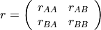- $r = \left(\begin{array}{cc} r_{AA} & r_{AB}\\r_{BA} & r_{BB}\end{array}\right)$ the covariance matrix, where index A (resp. B) refers to conditioning (resp. non-conditioning) index in the grid;
an unconditional simulation Z is updated into a conditional simulation ZCond as follows; let
- ZCond[A] = Zobs
- ZCond[B] = Z[B] + rBA * rAA^(-1) * (Zobs - Z[A])
i.e. the update consists in adding the kriging estimates of the residues to an unconditional simulation
- conditioningMethod=1 (method CondtioningA): the matrix M = rBA * rAA^(-1) is explicitly computed (warning: could require large amount of memory), then all the simulations are updated by a sum and a multiplication by the matrix M
- conditioningMethod=2 (method CondtioningB, default): for each simulation, the linear system rAA * x = Zobs - Z[A] is solved and then, the multiplication by rBA is done via fft
Note: parameter conditioningMethod is used only for conditional simulation
measureErrVar (float, default: 0.0) – measurement error variance; the error on conditioning data is assumed to follow the distrubution N(0, measureErrVar * I); i.e. rAA + measureErrVar * I is considered instead of rAA for stabilizing the linear system for this matrix; note: parameter measureErrVar is used only for conditional simulation
tolInvKappa (float, default: 1.e-10) – the simulation is stopped if the inverse of the condition number of rAA is above tolInvKappa; note: parameter tolInvKappa is used only for conditional simulation
verbose (int, default: 1) –
verbose mode, higher implies more printing (info):
- 0: no display
- 1: warnings
- 2: warnings + basic info
- 3 (or >2): all information
note that if an error occurred, it is raised
printInfo (bool, optional) –
deprecated, use verbose instead;
- if printInfo=False, verbose is set to 1 (overwritten)
- if printInfo=True, verbose is set to 3 (overwritten)
- if printInfo=None (default): not used
logger (logging.Logger, optional) – logger (see package logging) if specified, messages are written via logger (no print)

Returns:

grf – GRF realizations, with n1 = nx (= dimension) if crop=True, but n1 >= nx if crop=False; grf[i, j]: value of the i-th realisation at grid cell of index j

Return type:

2D array of shape (nreal, n1)

Notes

1. For reproducing covariance model, the dimension of GRF should be large enough; let K an integer such that K*`spacing` is greater or equal to the correlation range, then:

correlation accross opposite border should be removed by extending the domain sufficiently, i.e.

extensionMin >= K - 1
two cells could not be correlated simultaneously regarding both distances between them (with respect to the periodic grid), i.e. one should have

dimension+extensionMin >= 2*K - 1.

To sum up, extensionMin should be chosen such that

dimension+extensionMin >= max(dimension, K) + K - 1

i.e.

extensionMin >= max(K-1, 2*K-dimension-1)

For large data set:

conditioningMethod should be set to 2 for using FFT
measureErrVar can be set to a small positive value to stabilize the covariance matrix for conditioning locations (solving linear system).

Some mathematical details:

Discrete Fourier Transform (DFT) of a vector x of length N is given by

c = DFT(x) = F * x

where F is the N x N matrix with coefficients

F(j,k) = [exp(-i*2*pi*j*k/N)], 0 <= j,k <= N-1

We have

F^(-1) = 1/N * F^(*)

where ^(*) denotes the conjugate transpose.

Let

Q = 1/N^(1/2) * F

Then Q is unitary, i.e. Q^(-1) = Q^(*)

Then, we have

DFT = F = N^(1/2) * Q,

DFT^(-1) = 1/N * F^(*) = 1/N^(1/2) * Q^(*)

Using numpy package:

numpy.fft.fft() = DFT()

numpy.fft.ifft() = DFT^(-1)()

grf.grf2D(cov_model, dimension, spacing=(1.0, 1.0), origin=(0.0, 0.0), x=None, v=None, aggregate_data_op=None, aggregate_data_op_kwargs=None, mean=None, var=None, nreal=1, extensionMin=None, rangeFactorForExtensionMin=1.0, crop=True, method=3, conditioningMethod=2, measureErrVar=0.0, tolInvKappa=1e-10, verbose=1, printInfo=None, logger=None)

Generates Gaussian Random Fields (GRF) in 2D via Fast Fourier Transform (FFT).

In brief, the GRFs

are generated using the given covariance model (cov_model),
may have a specified mean (mean) and variance (var), which can be non stationary,
may be conditioned to location(s) x with value(s) v.

Parameters:

cov_model (geone.covModel.CovModel2D, or geone.covModel.CovModel1D, or function (callable)) – covariance model in 2D, or covariance model in 1D interpreted as an omni- directional covariance model, or directly a function of covariance (taking 2D lag vector(s) as argument)
dimension (2-tuple of ints) – dimension=(nx, ny), number of cells in the 2D simulation grid along each axis
spacing (2-tuple of floats, default: (1.0, 1.0)) – spacing=(sx, sy), cell size along each axis
origin (2-tuple of floats, default: (0.0, 0.0)) – origin=(ox, oy), origin of the 2D simulation grid (lower-left corner)
x (2D array of floats of shape (n, 2), optional) – data points locations, with n the number of data points, each row of x is the float coordinates of one data point; note: if n=1, a 1D array of shape (2,) is accepted
v (1D array of floats of shape (n,), optional) – data values at x (v[i] is the data value at x[i])
aggregate_data_op (str {'sgs', 'krige', 'min', 'max', 'mean', 'quantile', 'most_freq', 'random'}, optional) –
operation used to aggregate data points falling in the same grid cells
- if aggregate_data_op=’sgs’: function geone.covModel.sgs() is used with the covariance model cov_model given in arguments
- if aggregate_data_op=’krige’: function geone.covModel.krige() is used with the covariance model cov_model given in arguments
- if aggregate_data_op=’most_freq’: most frequent value is selected (smallest one if more than one value with the maximal frequence)
- if aggregate_data_op=’random’: value from a random point is selected
- otherwise: the function numpy.<aggregate_data_op> is used with the additional parameters given by aggregate_data_op_kwargs, note that, e.g. aggregate_data_op=’quantile’ requires the additional parameter q=<quantile_to_compute>
Note: if aggregate_data_op=’sgs’ or aggregate_data_op=’random’, the aggregation is done for each realization (simulation), i.e. each simulation on the grid starts with a new set of values in conditioning grid cells; if aggregate_data_op=’sgs’ or aggregate_data_op=’krige’, then cov_model must be a covariance model and not directly the covariance function

By default (None): aggregate_data_op=’sgs’ is used
aggregate_data_op_kwargs (dict, optional) – keyword arguments to be passed to geone.covModel.sgs, geone.covModel.krige, or numpy.<aggregate_data_op>, according to the parameter aggregate_data_op
mean (function (callable), or array-like of floats, or float, optional) –
kriging mean value:
- if a function: function of two arguments (xi, yi) that returns the mean at location (xi, yi)
- if array-like: its size must be equal to the number of grid cells (the array is reshaped if needed), mean values at grid cells (for non-stationary mean)
- if a float: same mean value at every grid cell
By default (None): the mean of data value (v) (0.0 if no data) is considered at every grid cell
var (function (callable), or array-like of floats, or float, optional) –
kriging variance value:
- if a function: function of two arguments (xi, yi) that returns the variance at location (xi, yi)
- if array-like: its size must be equal to the number of grid cells (the array is reshaped if needed), variance values at grid cells (for non-stationary variance)
- if a float: same variance value at every grid cell
By default (None): not used (use of covariance model only)
nreal (int, default: 1) – number of realization(s)
extensionMin (sequence of 2 ints, optional) –
minimal extension in cells along each axis (see note 1 below)

By default (None): minimal extension is automatically computed:
- based on the range of the covariance model, if cov_model is given as an instance of geone.covModel.CovModel1D (or geone.covModel.CovModel2D)
- set to (nx-1, ny-1), if cov_model is given as a function (callable)
rangeFactorForExtensionMin (float, default: 1.0) – factor by which the ranges of the covariance model are multiplied before computing the default minimal extension, if cov_model is given as an instance of geone.covModel.CovModel1D (or geone.covModel.CovModel2D) and if extensionMin=None (not used otherwise)
crop (bool, default: True) – indicates if the extended generated field (simulation) will be cropped to original dimension; note that crop=False is not valid with conditioning or non-stationary mean or non-stationary variance
method (int, default: 3) –
indicates which method is used to generate unconditional simulations; for each method the Discrete Fourier Transform (DFT) “lam” of the circulant embedding of the covariance matrix is used, and periodic and stationary GRFs are generated
- method=1 (method A): generate one GRF Z as follows:
  - generate one real gaussian white noise W
  - apply fft (or fft inverse) on W to get X
  - multiply X by “lam” (term by term)
  - apply fft inverse (or fft) to get Z
- method=2 (method B, not implemented!): generate one GRF Z as follows:
  - generate directly X (from method A)
  - multiply X by lam (term by term)
  - apply fft inverse (or fft) to get Z
- method=3 (method C, default): generate two independent GRFs Z1, Z2 as follows:
  - generate two independant real gaussian white noises W1, W2 and set W = W1 + i * W2
  - apply fft (or fft inverse) on W to get X
  - multiply X by “lam” (term by term)
  - apply fft inverse (or fft) to get Z, and set Z1 = Re(Z), Z2 = Im(Z); note: if nreal is odd, the last field is generated using method A
conditioningMethod (int, default: 2) –
indicates which method is used to update the simulations to account for conditioning data; let
- A: index of conditioning cells
- B: index of non-conditioning cells
- Zobs: vector of values of the unconditional simulation Z at conditioning cells
- $r = \left(\begin{array}{cc} r_{AA} & r_{AB}\\r_{BA} & r_{BB}\end{array}\right)$ the covariance matrix, where index A (resp. B) refers to conditioning (resp. non-conditioning) index in the grid;
an unconditional simulation Z is updated into a conditional simulation ZCond as follows; let
- ZCond[A] = Zobs
- ZCond[B] = Z[B] + rBA * rAA^(-1) * (Zobs - Z[A])
i.e. the update consists in adding the kriging estimates of the residues to an unconditional simulation
- conditioningMethod=1 (method CondtioningA): the matrix M = rBA * rAA^(-1) is explicitly computed (warning: could require large amount of memory), then all the simulations are updated by a sum and a multiplication by the matrix M
- conditioningMethod=2 (method CondtioningB, default): for each simulation, the linear system rAA * x = Zobs - Z[A] is solved and then, the multiplication by rBA is done via fft
Note: parameter conditioningMethod is used only for conditional simulation
measureErrVar (float, default: 0.0) – measurement error variance; the error on conditioning data is assumed to follow the distrubution N(0, measureErrVar * I); i.e. rAA + measureErrVar * I is considered instead of rAA for stabilizing the linear system for this matrix; note: parameter measureErrVar is used only for conditional simulation
tolInvKappa (float, default: 1.e-10) – the simulation is stopped if the inverse of the condition number of rAA is above tolInvKappa; note: parameter tolInvKappa is used only for conditional simulation
verbose (int, default: 1) –
verbose mode, higher implies more printing (info):
- 0: no display
- 1: warnings
- 2: warnings + basic info
- 3 (or >2): all information
note that if an error occurred, it is raised
printInfo (bool, optional) –
deprecated, use verbose instead;
- if printInfo=False, verbose is set to 1 (overwritten)
- if printInfo=True, verbose is set to 3 (overwritten)
- if printInfo=None (default): not used
logger (logging.Logger, optional) – logger (see package logging) if specified, messages are written via logger (no print)

Returns:

grf – GRF realizations, with

n1 = nx (= dimension[0]), n2 = ny (= dimension[1]), if crop=True,
but n1 >= nx, n2 >= ny if crop=False

grf[i, iy, ix]: value of the i-th realisation at grid cell of index ix (resp. iy) along x (resp. y) axis

Return type:

3D array of shape (nreal, n2, n1)

Notes

1. For reproducing covariance model, the dimension of GRF should be large enough; let K an integer such that K*`spacing` is greater or equal to the correlation range, then:

correlation accross opposite border should be removed by extending the domain sufficiently, i.e.

extensionMin >= K - 1
two cells could not be correlated simultaneously regarding both distances between them (with respect to the periodic grid), i.e. one should have

dimension+extensionMin >= 2*K - 1.

To sum up, extensionMin should be chosen such that

dimension+extensionMin >= max(dimension, K) + K - 1

i.e.

extensionMin >= max(K-1, 2*K-dimension-1)

For large data set:

conditioningMethod should be set to 2 for using FFT
measureErrVar can be set to a small positive value to stabilize the covariance matrix for conditioning locations (solving linear system).

Some mathematical details:

Discrete Fourier Transform (DFT) of an array x of dim N1 x N2 is given by

c = DFT(x) = F * x

where F is the the (N1*N2) x (N1*N2) matrix with coefficients

F(j,k) = [exp( -i*2*pi*(j^t*k)/(N1*N2) )], j=(j1,j2), k=(k1,k2) in G,

and

G = {n=(n1,n2), 0 <= n1 <= N1-1, 0 <= n2 <= N2-1}

denotes the indices grid and where we use the bijection

(n1,n2) in G -> n1 + n2 * N1 in {0,…,N1*N2-1},

between the multiple-indices and the single indices.

With N = N1*N2, we have

F^(-1) = 1/N * F^(*)

where ^(*) denotes the conjugate transpose.

Let

Q = 1/N^(1/2) * F

Then Q is unitary, i.e. Q^(-1) = Q^(*)

Then, we have

DFT = F = N^(1/2) * Q,

DFT^(-1) = 1/N * F^(*) = 1/N^(1/2) * Q^(*)

Using numpy package:

numpy.fft.fft2() = DFT()

numpy.fft.ifft2() = DFT^(-1)()

grf.grf3D(cov_model, dimension, spacing=(1.0, 1.0, 1.0), origin=(0.0, 0.0, 0.0), x=None, v=None, aggregate_data_op=None, aggregate_data_op_kwargs=None, mean=None, var=None, nreal=1, extensionMin=None, rangeFactorForExtensionMin=1.0, crop=True, method=3, conditioningMethod=2, measureErrVar=0.0, tolInvKappa=1e-10, verbose=1, printInfo=None, logger=None)

Generates Gaussian Random Fields (GRF) in 3D via Fast Fourier Transform (FFT).

In brief, the GRFs

are generated using the given covariance model (cov_model),
may have a specified mean (mean) and variance (var), which can be non stationary,
may be conditioned to location(s) x with value(s) v.

Parameters:

cov_model (geone.covModel.CovModel3D, or geone.covModel.CovModel1D, or function (callable)) – covariance model in 3D, or covariance model in 1D interpreted as an omni- directional covariance model, or directly a function of covariance (taking 3D lag vector(s) as argument)
dimension (3-tuple of ints) – dimension=(nx, ny, nz), number of cells in the 3D simulation grid along each axis
spacing (3-tuple of floats, default: (1.0,1.0, 1.0)) – spacing=(sx, sy, sz), cell size along each axis
origin (3-tuple of floats, default: (0.0, 0.0, 0.0)) – origin=(ox, oy, oz), origin of the 3D simulation grid (bottom-lower-left corner)
x (2D array of floats of shape (n, 3), optional) – data points locations, with n the number of data points, each row of x is the float coordinates of one data point; note: if n=1, a 1D array of shape (3,) is accepted
v (1D array of floats of shape (n,), optional) – data values at x (v[i] is the data value at x[i])
aggregate_data_op (str {'sgs', 'krige', 'min', 'max', 'mean', 'quantile', 'most_freq', 'random'}, optional) –
operation used to aggregate data points falling in the same grid cells
- if aggregate_data_op=’sgs’: function geone.covModel.sgs() is used with the covariance model cov_model given in arguments
- if aggregate_data_op=’krige’: function geone.covModel.krige() is used with the covariance model cov_model given in arguments
- if aggregate_data_op=’most_freq’: most frequent value is selected (smallest one if more than one value with the maximal frequence)
- if aggregate_data_op=’random’: value from a random point is selected
- otherwise: the function numpy.<aggregate_data_op> is used with the additional parameters given by aggregate_data_op_kwargs, note that, e.g. aggregate_data_op=’quantile’ requires the additional parameter q=<quantile_to_compute>
Note: if aggregate_data_op=’sgs’ or aggregate_data_op=’random’, the aggregation is done for each realization (simulation), i.e. each simulation on the grid starts with a new set of values in conditioning grid cells; if aggregate_data_op=’sgs’ or aggregate_data_op=’krige’, then cov_model must be a covariance model and not directly the covariance function

By default (None): aggregate_data_op=’sgs’ is used
aggregate_data_op_kwargs (dict, optional) – keyword arguments to be passed to geone.covModel.sgs, geone.covModel.krige, or numpy.<aggregate_data_op>, according to the parameter aggregate_data_op
mean (function (callable), or array-like of floats, or float, optional) –
kriging mean value:
- if a function: function of three arguments (xi, yi, zi) that returns the mean at location (xi, yi, zi)
- if array-like: its size must be equal to the number of grid cells (the array is reshaped if needed), mean values at grid cells (for non-stationary mean)
- if a float: same mean value at every grid cell
By default (None): the mean of data value (v) (0.0 if no data) is considered at every grid cell
var (function (callable), or array-like of floats, or float, optional) –
kriging variance value:
- if a function: function of three arguments (xi, yi, yi) that returns the variance at location (xi, yi, zi)
- if array-like: its size must be equal to the number of grid cells (the array is reshaped if needed), variance values at grid cells (for non-stationary variance)
- if a float: same variance value at every grid cell
By default (None): not used (use of covariance model only)
nreal (int, default: 1) – number of realization(s)
extensionMin (sequence of 3 ints, optional) –
minimal extension in cells along each axis (see note 1 below)

By default (None): minimal extension is automatically computed:
- based on the range of the covariance model, if cov_model is given as an instance of geone.covModel.CovModel1D (or geone.covModel.CovModel3D)
- set to (nx-1, ny-1, nz-1), if cov_model is given as a function (callable)
rangeFactorForExtensionMin (float, default: 1.0) – factor by which the ranges of the covariance model are multiplied before computing the default minimal extension, if cov_model is given as an instance of geone.covModel.CovModel1D (or geone.covModel.CovModel3D) and if extensionMin=None (not used otherwise)
crop (bool, default: True) – indicates if the extended generated field (simulation) will be cropped to original dimension; note that crop=False is not valid with conditioning or non-stationary mean or non-stationary variance
method (int, default: 3) –
indicates which method is used to generate unconditional simulations; for each method the Discrete Fourier Transform (DFT) “lam” of the circulant embedding of the covariance matrix is used, and periodic and stationary GRFs are generated
- method=1 (method A): generate one GRF Z as follows:
  - generate one real gaussian white noise W
  - apply fft (or fft inverse) on W to get X
  - multiply X by “lam” (term by term)
  - apply fft inverse (or fft) to get Z
- method=2 (method B, not implemented!): generate one GRF Z as follows:
  - generate directly X (from method A)
  - multiply X by lam (term by term)
  - apply fft inverse (or fft) to get Z
- method=3 (method C, default): generate two independent GRFs Z1, Z2 as follows:
  - generate two independant real gaussian white noises W1, W2 and set W = W1 + i * W2
  - apply fft (or fft inverse) on W to get X
  - multiply X by “lam” (term by term)
  - apply fft inverse (or fft) to get Z, and set Z1 = Re(Z), Z2 = Im(Z); note: if nreal is odd, the last field is generated using method A
conditioningMethod (int, default: 2) –
indicates which method is used to update the simulations to account for conditioning data; let
- A: index of conditioning cells
- B: index of non-conditioning cells
- Zobs: vector of values of the unconditional simulation Z at conditioning cells
- $r = \left(\begin{array}{cc} r_{AA} & r_{AB}\\r_{BA} & r_{BB}\end{array}\right)$ the covariance matrix, where index A (resp. B) refers to conditioning (resp. non-conditioning) index in the grid;
an unconditional simulation Z is updated into a conditional simulation ZCond as follows; let
- ZCond[A] = Zobs
- ZCond[B] = Z[B] + rBA * rAA^(-1) * (Zobs - Z[A])
i.e. the update consists in adding the kriging estimates of the residues to an unconditional simulation
- conditioningMethod=1 (method CondtioningA): the matrix M = rBA * rAA^(-1) is explicitly computed (warning: could require large amount of memory), then all the simulations are updated by a sum and a multiplication by the matrix M
- conditioningMethod=2 (method CondtioningB, default): for each simulation, the linear system rAA * x = Zobs - Z[A] is solved and then, the multiplication by rBA is done via fft
Note: parameter conditioningMethod is used only for conditional simulation
measureErrVar (float, default: 0.0) – measurement error variance; the error on conditioning data is assumed to follow the distrubution N(0, measureErrVar * I); i.e. rAA + measureErrVar * I is considered instead of rAA for stabilizing the linear system for this matrix; note: parameter measureErrVar is used only for conditional simulation
tolInvKappa (float, default: 1.e-10) – the simulation is stopped if the inverse of the condition number of rAA is above tolInvKappa; note: parameter tolInvKappa is used only for conditional simulation
verbose (int, default: 1) –
verbose mode, higher implies more printing (info):
- 0: no display
- 1: warnings
- 2: warnings + basic info
- 3 (or >2): all information
note that if an error occurred, it is raised
printInfo (bool, optional) –
deprecated, use verbose instead;
- if printInfo=False, verbose is set to 1 (overwritten)
- if printInfo=True, verbose is set to 3 (overwritten)
- if printInfo=None (default): not used
logger (logging.Logger, optional) – logger (see package logging) if specified, messages are written via logger (no print)

Returns:

grf – GRF realizations, with

n1 = nx (= dimension[0]), n2 = ny (= dimension[1]), n3 = nz (= dimension[2]), if crop=True,
but n1 >= nx, n2 >= ny, n3 >= nz if crop=False;

grf[i, iz, iy, ix]: value of the i-th realisation at grid cell of index ix (resp. iy, iz) along x (resp. y, z) axis

Return type:

4D array of shape (nreal, n3, n2, n1)

Notes

1. For reproducing covariance model, the dimension of GRF should be large enough; let K an integer such that K*`spacing` is greater or equal to the correlation range, then:

correlation accross opposite border should be removed by extending the domain sufficiently, i.e.

extensionMin >= K - 1
two cells could not be correlated simultaneously regarding both distances between them (with respect to the periodic grid), i.e. one should have

dimension+extensionMin >= 2*K - 1.

To sum up, extensionMin should be chosen such that

dimension+extensionMin >= max(dimension, K) + K - 1

i.e.

extensionMin >= max(K-1, 2*K-dimension-1)

For large data set:

conditioningMethod should be set to 2 for using FFT
measureErrVar can be set to a small positive value to stabilize the covariance matrix for conditioning locations (solving linear system).

Some mathematical details:

Discrete Fourier Transform (DFT) of an array x of dim N1 x N2 x N3 is given by

c = DFT(x) = F * x

where F is the the (N1*N2*N3) x (N1*N2*N3) matrix with coefficients

F(j,k) = [exp( -i*2*pi*(j^t*k)/(N1*N2*N3) )], j=(j1,j2,j3), k=(k1,k2,k3) in G,

and

G = {n=(n1,n2,n3), 0 <= n1 <= N1-1, 0 <= n2 <= N2-1, 0 <= n3 <= N3-1}

denotes the indices grid and where we use the bijection

(n1,n2,n3) in G -> n1 + n2 * N1 + n3 * N1 * N2 in {0,…,N1*N2*N3-1},

between the multiple-indices and the single indices.

With N = N1*N2*N3, we have

F^(-1) = 1/N * F^(*)

where ^(*) denotes the conjugate transpose.

Let

Q = 1/N^(1/2) * F

Then Q is unitary, i.e. Q^(-1) = Q^(*)

Then, we have

DFT = F = N^(1/2) * Q,

DFT^(-1) = 1/N * F^(*) = 1/N^(1/2) * Q^(*)

Using numpy package:

numpy.fft.fftn() = DFT()

numpy.fft.ifftn() = DFT^(-1)()

grf.krige1D(cov_model, dimension, spacing=1.0, origin=0.0, x=None, v=None, aggregate_data_op=None, aggregate_data_op_kwargs=None, mean=None, var=None, extensionMin=None, rangeFactorForExtensionMin=1.0, conditioningMethod=1, measureErrVar=0.0, tolInvKappa=1e-10, computeKrigSD=True, verbose=1, printInfo=None, logger=None)

Computes kriging estimates and standard deviations in 1D via FFT.

It is a simple kriging

of value(s) v at location(s) x,
based on the given covariance model (cov_model),
it may account for a specified mean (mean) and variance (var), which can be non stationary.

Parameters:

cov_model (geone.covModel.CovModel1D, or function (callable)) – covariance model in 1D or directly a function of covariance
dimension (int) – dimension=nx, number of cells in the 1D simulation grid
spacing (float, default: 1.0) – spacing=sx, cell size
origin (float, default: 0.0) – origin=ox, origin of the 1D simulation grid (left border)
x (1D array-like of floats, optional) – data points locations (float coordinates); note: if one point, a float is accepted
v (1D array-like of floats, optional) – data values at x (v[i] is the data value at x[i]), array of same length as x (or float if one point)
aggregate_data_op (str {'krige', 'min', 'max', 'mean', 'quantile', 'most_freq'}, optional) –
operation used to aggregate data points falling in the same grid cells
- if aggregate_data_op=’krige’: function geone.covModel.krige() is used with the covariance model cov_model given in arguments
- if aggregate_data_op=’most_freq’: most frequent value is selected (smallest one if more than one value with the maximal frequence)
- otherwise: the function numpy.<aggregate_data_op> is used with the additional parameters given by aggregate_data_op_kwargs, note that, e.g. aggregate_data_op=’quantile’ requires the additional parameter q=<quantile_to_compute>
Note: if aggregate_data_op=’krige’, then cov_model must be a covariance model and not directly the covariance function

By default (None): aggregate_data_op=’krige’ is used
aggregate_data_op_kwargs (dict, optional) – keyword arguments to be passed to geone.covModel.krige, geone.covModel.krige, or numpy.<aggregate_data_op>, according to the parameter aggregate_data_op
mean (function (callable), or array-like of floats, or float, optional) –
kriging mean value:
- if a function: function of one argument (xi) that returns the mean at location xi
- if array-like: its size must be equal to the number of grid cells (the array is reshaped if needed), mean values at grid cells (for non-stationary mean)
- if a float: same mean value at every grid cell
By default (None): the mean of data value (v) (0.0 if no data) is considered at every grid cell
var (function (callable), or array-like of floats, or float, optional) –
kriging variance value:
- if a function: function of one argument (xi) that returns the variance at location xi
- if array-like: its size must be equal to the number of grid cells (the array is reshaped if needed), variance values at grid cells (for non-stationary variance)
- if a float: same variance value at every grid cell
By default (None): not used (use of covariance model only)
extensionMin (int, optional) –
minimal extension in cells (see note 1 below)

By default (None): minimal extension is automatically computed:
- based on the range of the covariance model, if cov_model is given as an instance of geone.covModel.CovModel1D)
- set to nx-1, if cov_model is given as a function (callable)
rangeFactorForExtensionMin (float, default: 1.0) – factor by which the range of the covariance model is multiplied before computing the default minimal extension, if cov_model is given as an instance of geone.covModel.CovModel1D) and if extensionMin=None (not used otherwise)
conditioningMethod (int, default: 1) –
indicates which method is used to update the simulations to account for conditioning data; let
- A: index of conditioning cells
- B: index of non-conditioning cells
- $r = \left(\begin{array}{cc} r_{AA} & r_{AB}\\r_{BA} & r_{BB}\end{array}\right)$ the covariance matrix, where index A (resp. B) refers to conditioning (resp. non-conditioning) index in the grid;
then, thre kriging estimates and kriging variances are
- krig[B] = mean + rBA * rAA^(-1) * (v - mean)
- krigVar[B] = diag(rBB - rBA * rAA^(-1) * rAB)
and the computation is done according to conditioningMethod:
- conditioningMethod=1 (method CondtioningA, default): the matrices rBA, RAA^(-1) are explicitly computed (warning: could require large amount of memory)
- conditioningMethod=2 (method CondtioningB): for kriging estimates, the linear system rAA * y = (v - mean) is solved, and then mean + rBA*y is computed; for kriging variances, for each column u[j] of rAB, the linear system rAA * y = u[j] is solved, and then rBB[j,j] - y^t*y is computed
Note: set conditioningMethod=2 if unable to allocate memory
measureErrVar (float, default: 0.0) – measurement error variance; the error on conditioning data is assumed to follow the distrubution N(0, measureErrVar * I); i.e. rAA + measureErrVar * I is considered instead of rAA for stabilizing the linear system for this matrix
tolInvKappa (float, default: 1.e-10) – the computation is stopped if the inverse of the condition number of rAA is above tolInvKappa
computeKrigSD (bool, default: True) – indicates if the kriging standard deviations are computed
verbose (int, default: 2) –
verbose mode, higher implies more printing (info):
- 0: no display
- 1: warnings
- 2: warnings + basic info
- 3 (or >2): all information
note that if an error occurred, it is raised
printInfo (bool, optional) –
deprecated, use verbose instead;
- if printInfo=False, verbose is set to 1 (overwritten)
- if printInfo=True, verbose is set to 3 (overwritten)
- if printInfo=None (default): not used
logger (logging.Logger, optional) – logger (see package logging) if specified, messages are written via logger (no print)

Returns:

krig (1D array of shape (nx,)) – kriging estimates, with nx (= dimension); krig[j]: value at grid cell of index j
krigSD (1D array of shape (nx,), optional) – kriging standard deviations, with nx (= dimension); krigSD[j]: value at grid cell of index j; returned if computeKrigSD=True

Notes

1. For reproducing covariance model, the dimension of GRF should be large enough; let K an integer such that K*`spacing` is greater or equal to the correlation range, then:

correlation accross opposite border should be removed by extending the domain sufficiently, i.e.

extensionMin >= K - 1
two cells could not be correlated simultaneously regarding both distances between them (with respect to the periodic grid), i.e. one should have

dimension+extensionMin >= 2*K - 1.

To sum up, extensionMin should be chosen such that

dimension+extensionMin >= max(dimension, K) + K - 1

i.e.

extensionMin >= max(K-1, 2*K-dimension-1)

For large data set:

conditioningMethod should be set to 2 for using FFT
measureErrVar can be set to a small positive value to stabilize the covariance matrix for conditioning locations (solving linear system).

Some mathematical details:

Discrete Fourier Transform (DFT) of a vector x of length N is given by

c = DFT(x) = F * x

where F is the N x N matrix with coefficients

F(j,k) = [exp(-i*2*pi*j*k/N)], 0 <= j,k <= N-1

We have

F^(-1) = 1/N * F^(*)

where ^(*) denotes the conjugate transpose.

Let

Q = 1/N^(1/2) * F

Then Q is unitary, i.e. Q^(-1) = Q^(*)

Then, we have

DFT = F = N^(1/2) * Q,

DFT^(-1) = 1/N * F^(*) = 1/N^(1/2) * Q^(*)

Using numpy package:

numpy.fft.fft() = DFT()

numpy.fft.ifft() = DFT^(-1)()

grf.krige2D(cov_model, dimension, spacing=(1.0, 1.0), origin=(0.0, 0.0), x=None, v=None, aggregate_data_op=None, aggregate_data_op_kwargs=None, mean=None, var=None, extensionMin=None, rangeFactorForExtensionMin=1.0, conditioningMethod=1, measureErrVar=0.0, tolInvKappa=1e-10, computeKrigSD=True, verbose=1, printInfo=None, logger=None)

Computes kriging estimates and standard deviations in 2D via FFT.

It is a simple kriging

of value(s) v at location(s) x,
based on the given covariance model (cov_model),
it may account for a specified mean (mean) and variance (var), which can be non stationary.

Parameters:

cov_model (geone.covModel.CovModel2D, or geone.covModel.CovModel1D, or function (callable)) – covariance model in 2D, or covariance model in 1D interpreted as an omni- directional covariance model, or directly a function of covariance (taking 2D lag vector(s) as argument)
dimension (2-tuple of ints) – dimension=(nx, ny), number of cells in the 2D simulation grid along each axis
spacing (2-tuple of floats, default: (1.0, 1.0)) – spacing=(sx, sy), cell size along each axis
origin (2-tuple of floats, default: (0.0, 0.0)) – origin=(ox, oy), origin of the 2D simulation grid (lower-left corner)
x (2D array of floats of shape (n, 2), optional) – data points locations, with n the number of data points, each row of x is the float coordinates of one data point; note: if n=1, a 1D array of shape (2,) is accepted
v (1D array of floats of shape (n,), optional) – data values at x (v[i] is the data value at x[i])
aggregate_data_op (str {'krige', 'min', 'max', 'mean', 'quantile', 'most_freq'}, optional) –
operation used to aggregate data points falling in the same grid cells
- if aggregate_data_op=’krige’: function geone.covModel.krige() is used with the covariance model cov_model given in arguments
- if aggregate_data_op=’most_freq’: most frequent value is selected (smallest one if more than one value with the maximal frequence)
- otherwise: the function numpy.<aggregate_data_op> is used with the additional parameters given by aggregate_data_op_kwargs, note that, e.g. aggregate_data_op=’quantile’ requires the additional parameter q=<quantile_to_compute>
Note: if aggregate_data_op=’krige’, then cov_model must be a covariance model and not directly the covariance function

By default (None): aggregate_data_op=’krige’ is used
aggregate_data_op_kwargs (dict, optional) – keyword arguments to be passed to geone.covModel.krige, geone.covModel.krige, or numpy.<aggregate_data_op>, according to the parameter aggregate_data_op
mean (function (callable), or array-like of floats, or float, optional) –
kriging mean value:
- if a function: function of two arguments (xi, yi) that returns the mean at location (xi, yi)
- if array-like: its size must be equal to the number of grid cells (the array is reshaped if needed), mean values at grid cells (for non-stationary mean)
- if a float: same mean value at every grid cell
By default (None): the mean of data value (v) (0.0 if no data) is considered at every grid cell
var (function (callable), or array-like of floats, or float, optional) –
kriging variance value:
- if a function: function of two arguments (xi, yi) that returns the variance at location (xi, yi)
- if array-like: its size must be equal to the number of grid cells (the array is reshaped if needed), variance values at grid cells (for non-stationary variance)
- if a float: same variance value at every grid cell
By default (None): not used (use of covariance model only)
extensionMin (sequence of 2 ints, optional) –
minimal extension in cells along each axis (see note 1 below)

By default (None): minimal extension is automatically computed:
- based on the range of the covariance model, if cov_model is given as an instance of geone.covModel.CovModel1D (or geone.covModel.CovModel2D)
- set to (nx-1, ny-1), if cov_model is given as a function (callable)
rangeFactorForExtensionMin (float, default: 1.0) – factor by which the ranges of the covariance model are multiplied before computing the default minimal extension, if cov_model is given as an instance of geone.covModel.CovModel1D (or geone.covModel.CovModel2D) and if extensionMin=None (not used otherwise)
conditioningMethod (int, default: 1) –
indicates which method is used to update the simulations to account for conditioning data; let
- A: index of conditioning cells
- B: index of non-conditioning cells
- $r = \left(\begin{array}{cc} r_{AA} & r_{AB}\\r_{BA} & r_{BB}\end{array}\right)$ the covariance matrix, where index A (resp. B) refers to conditioning (resp. non-conditioning) index in the grid;
then, thre kriging estimates and kriging variances are
- krig[B] = mean + rBA * rAA^(-1) * (v - mean)
- krigVar[B] = diag(rBB - rBA * rAA^(-1) * rAB)
and the computation is done according to conditioningMethod:
- conditioningMethod=1 (method CondtioningA, default): the matrices rBA, RAA^(-1) are explicitly computed (warning: could require large amount of memory)
- conditioningMethod=2 (method CondtioningB): for kriging estimates, the linear system rAA * y = (v - mean) is solved, and then mean + rBA*y is computed; for kriging variances, for each column u[j] of rAB, the linear system rAA * y = u[j] is solved, and then rBB[j,j] - y^t*y is computed
Note: set conditioningMethod=2 if unable to allocate memory
measureErrVar (float, default: 0.0) – measurement error variance; the error on conditioning data is assumed to follow the distrubution N(0, measureErrVar * I); i.e. rAA + measureErrVar * I is considered instead of rAA for stabilizing the linear system for this matrix
tolInvKappa (float, default: 1.e-10) – the computation is stopped if the inverse of the condition number of rAA is above tolInvKappa
computeKrigSD (bool, default: True) – indicates if the kriging standard deviations are computed
verbose (int, default: 1) –
verbose mode, higher implies more printing (info):
- 0: no display
- 1: warnings
- 2: warnings + basic info
- 3 (or >2): all information
note that if an error occurred, it is raised
printInfo (bool, optional) –
deprecated, use verbose instead;
- if printInfo=False, verbose is set to 1 (overwritten)
- if printInfo=True, verbose is set to 3 (overwritten)
- if printInfo=None (default): not used
logger (logging.Logger, optional) – logger (see package logging) if specified, messages are written via logger (no print)

Returns:

krig (2D array of shape (ny, nx)) – kriging estimates, with (nx, ny) (= dimension); krig[iy, ix]: value at grid cell of index ix (resp. iy) along x (resp. y) axis
krigSD (2D array of shape (ny, nx), optional) – kriging standard deviations, with (nx, ny) (= dimension); krigSD[iy, ix]: value at grid cell of index ix (resp. iy) along x (resp. y) axis; returned if computeKrigSD=True

Notes

1. For reproducing covariance model, the dimension of GRF should be large enough; let K an integer such that K*`spacing` is greater or equal to the correlation range, then:

correlation accross opposite border should be removed by extending the domain sufficiently, i.e.

extensionMin >= K - 1
two cells could not be correlated simultaneously regarding both distances between them (with respect to the periodic grid), i.e. one should have

dimension+extensionMin >= 2*K - 1.

To sum up, extensionMin should be chosen such that

dimension+extensionMin >= max(dimension, K) + K - 1

i.e.

extensionMin >= max(K-1, 2*K-dimension-1)

For large data set:

conditioningMethod should be set to 2 for using FFT
measureErrVar can be set to a small positive value to stabilize the covariance matrix for conditioning locations (solving linear system).

Some mathematical details:

Discrete Fourier Transform (DFT) of an array x of dim N1 x N2 is given by

c = DFT(x) = F * x

where F is the the (N1*N2) x (N1*N2) matrix with coefficients

F(j,k) = [exp( -i*2*pi*(j^t*k)/(N1*N2) )], j=(j1,j2), k=(k1,k2) in G,

and

G = {n=(n1,n2), 0 <= n1 <= N1-1, 0 <= n2 <= N2-1}

denotes the indices grid and where we use the bijection

(n1,n2) in G -> n1 + n2 * N1 in {0,…,N1*N2-1},

between the multiple-indices and the single indices.

With N = N1*N2, we have

F^(-1) = 1/N * F^(*)

where ^(*) denotes the conjugate transpose.

Let

Q = 1/N^(1/2) * F

Then Q is unitary, i.e. Q^(-1) = Q^(*)

Then, we have

DFT = F = N^(1/2) * Q,

DFT^(-1) = 1/N * F^(*) = 1/N^(1/2) * Q^(*)

Using numpy package:

numpy.fft.fft2() = DFT()

numpy.fft.ifft2() = DFT^(-1)()

grf.krige3D(cov_model, dimension, spacing=(1.0, 1.0, 1.0), origin=(0.0, 0.0, 0.0), x=None, v=None, aggregate_data_op=None, aggregate_data_op_kwargs=None, mean=None, var=None, extensionMin=None, rangeFactorForExtensionMin=1.0, conditioningMethod=1, measureErrVar=0.0, tolInvKappa=1e-10, computeKrigSD=True, verbose=1, printInfo=None, logger=None)

Computes kriging estimates and standard deviations in 3D via FFT.

It is a simple kriging

of value(s) v at location(s) x,
based on the given covariance model (cov_model),
it may account for a specified mean (mean) and variance (var), which can be non stationary.

Parameters:

cov_model (geone.covModel.CovModel3D, or geone.covModel.CovModel1D, or function (callable)) – covariance model in 3D, or covariance model in 1D interpreted as an omni- directional covariance model, or directly a function of covariance (taking 3D lag vector(s) as argument)
dimension (3-tuple of ints) – dimension=(nx, ny, nz), number of cells in the 3D simulation grid along each axis
spacing (3-tuple of floats, default: (1.0,1.0, 1.0)) – spacing=(sx, sy, sz), cell size along each axis
origin (3-tuple of floats, default: (0.0, 0.0, 0.0)) – origin=(ox, oy, oz), origin of the 3D simulation grid (bottom-lower-left corner)
x (2D array of floats of shape (n, 3), optional) – data points locations, with n the number of data points, each row of x is the float coordinates of one data point; note: if n=1, a 1D array of shape (3,) is accepted
v (1D array of floats of shape (n,), optional) – data values at x (v[i] is the data value at x[i])
aggregate_data_op (str {'krige', 'min', 'max', 'mean', 'quantile', 'most_freq'}, optional) –
operation used to aggregate data points falling in the same grid cells
- if aggregate_data_op=’krige’: function geone.covModel.krige() is used with the covariance model cov_model given in arguments
- if aggregate_data_op=’most_freq’: most frequent value is selected (smallest one if more than one value with the maximal frequence)
- otherwise: the function numpy.<aggregate_data_op> is used with the additional parameters given by aggregate_data_op_kwargs, note that, e.g. aggregate_data_op=’quantile’ requires the additional parameter q=<quantile_to_compute>
Note: if aggregate_data_op=’krige’, then cov_model must be a covariance model and not directly the covariance function

By default (None): aggregate_data_op=’krige’ is used
aggregate_data_op_kwargs (dict, optional) – keyword arguments to be passed to geone.covModel.krige, geone.covModel.krige, or numpy.<aggregate_data_op>, according to the parameter aggregate_data_op
aggregate_data_op_kwargs – keyword arguments to be passed to geone.covModel.krige or numpy.<aggregate_data_op>, according to the parameter aggregate_data_op
mean (function (callable), or array-like of floats, or float, optional) –
kriging mean value:
- if a function: function of three arguments (xi, yi, zi) that returns the mean at location (xi, yi, zi)
- if array-like: its size must be equal to the number of grid cells (the array is reshaped if needed), mean values at grid cells (for non-stationary mean)
- if a float: same mean value at every grid cell
By default (None): the mean of data value (v) (0.0 if no data) is considered at every grid cell
var (function (callable), or array-like of floats, or float, optional) –
kriging variance value:
- if a function: function of three arguments (xi, yi, yi) that returns the variance at location (xi, yi, zi)
- if array-like: its size must be equal to the number of grid cells (the array is reshaped if needed), variance values at grid cells (for non-stationary variance)
- if a float: same variance value at every grid cell
By default (None): not used (use of covariance model only)
extensionMin (sequence of 3 ints, optional) –
minimal extension in cells along each axis (see note 1 below)

By default (None): minimal extension is automatically computed:
- based on the range of the covariance model, if cov_model is given as an instance of geone.covModel.CovModel1D (or geone.covModel.CovModel3D)
- set to (nx-1, ny-1, nz-1), if cov_model is given as a function (callable)
rangeFactorForExtensionMin (float, default: 1.0) – factor by which the ranges of the covariance model are multiplied before computing the default minimal extension, if cov_model is given as an instance of geone.covModel.CovModel1D (or geone.covModel.CovModel3D) and if extensionMin=None (not used otherwise)
conditioningMethod (int, default: 1) –
indicates which method is used to update the simulations to account for conditioning data; let
- A: index of conditioning cells
- B: index of non-conditioning cells
- $r = \left(\begin{array}{cc} r_{AA} & r_{AB}\\r_{BA} & r_{BB}\end{array}\right)$ the covariance matrix, where index A (resp. B) refers to conditioning (resp. non-conditioning) index in the grid;
then, thre kriging estimates and kriging variances are
- krig[B] = mean + rBA * rAA^(-1) * (v - mean)
- krigVar[B] = diag(rBB - rBA * rAA^(-1) * rAB)
and the computation is done according to conditioningMethod:
- conditioningMethod=1 (method CondtioningA, default): the matrices rBA, RAA^(-1) are explicitly computed (warning: could require large amount of memory)
- conditioningMethod=2 (method CondtioningB): for kriging estimates, the linear system rAA * y = (v - mean) is solved, and then mean + rBA*y is computed; for kriging variances, for each column u[j] of rAB, the linear system rAA * y = u[j] is solved, and then rBB[j,j] - y^t*y is computed
Note: set conditioningMethod=2 if unable to allocate memory
measureErrVar (float, default: 0.0) – measurement error variance; the error on conditioning data is assumed to follow the distrubution N(0, measureErrVar * I); i.e. rAA + measureErrVar * I is considered instead of rAA for stabilizing the linear system for this matrix
tolInvKappa (float, default: 1.e-10) – the computation is stopped if the inverse of the condition number of rAA is above tolInvKappa
computeKrigSD (bool, default: True) – indicates if the kriging standard deviations are computed
verbose (int, default: 1) –
verbose mode, higher implies more printing (info):
- 0: no display
- 1: warnings
- 2: warnings + basic info
- 3 (or >2): all information
note that if an error occurred, it is raised
printInfo (bool, optional) –
deprecated, use verbose instead;
- if printInfo=False, verbose is set to 1 (overwritten)
- if printInfo=True, verbose is set to 3 (overwritten)
- if printInfo=None (default): not used
logger (logging.Logger, optional) – logger (see package logging) if specified, messages are written via logger (no print)

Returns:

krig (3D array of shape (nz, ny, nx)) – kriging estimates, with (nx, ny, nz) (= dimension); krig[iz, iy, ix]: value at grid cell of index ix (resp. iy, iz) along x (resp. y, z) axis
krigSD (3D array of shape (nz, ny, nx), optional) – kriging standard deviations, with (nx, ny, nz) (= dimension); krigSD[iz, iy, ix]: value at grid cell of index ix (resp. iy, iz) along x (resp. y, z) axis; returned if computeKrigSD=True

Notes

1. For reproducing covariance model, the dimension of GRF should be large enough; let K an integer such that K*`spacing` is greater or equal to the correlation range, then:

correlation accross opposite border should be removed by extending the domain sufficiently, i.e.

extensionMin >= K - 1
two cells could not be correlated simultaneously regarding both distances between them (with respect to the periodic grid), i.e. one should have

dimension+extensionMin >= 2*K - 1.

To sum up, extensionMin should be chosen such that

dimension+extensionMin >= max(dimension, K) + K - 1

i.e.

extensionMin >= max(K-1, 2*K-dimension-1)

For large data set:

conditioningMethod should be set to 2 for using FFT
measureErrVar can be set to a small positive value to stabilize the covariance matrix for conditioning locations (solving linear system).

Some mathematical details:

Discrete Fourier Transform (DFT) of an array x of dim N1 x N2 x N3 is given by

c = DFT(x) = F * x

where F is the the (N1*N2*N3) x (N1*N2*N3) matrix with coefficients

F(j,k) = [exp( -i*2*pi*(j^t*k)/(N1*N2*N3) )], j=(j1,j2,j3), k=(k1,k2,k3) in G,

and

G = {n=(n1,n2,n3), 0 <= n1 <= N1-1, 0 <= n2 <= N2-1, 0 <= n3 <= N3-1}

denotes the indices grid and where we use the bijection

(n1,n2,n3) in G -> n1 + n2 * N1 + n3 * N1 * N2 in {0,…,N1*N2*N3-1},

between the multiple-indices and the single indices.

With N = N1*N2*N3, we have

F^(-1) = 1/N * F^(*)

where ^(*) denotes the conjugate transpose.

Let

Q = 1/N^(1/2) * F

Then Q is unitary, i.e. Q^(-1) = Q^(*)

Then, we have

DFT = F = N^(1/2) * Q,

DFT^(-1) = 1/N * F^(*) = 1/N^(1/2) * Q^(*)

Using numpy package:

numpy.fft.fftn() = DFT()

numpy.fft.ifftn() = DFT^(-1)()

img

Module for “images” and “point sets”, and relative functions.

class img.Img(nx=1, ny=1, nz=1, sx=1.0, sy=1.0, sz=1.0, ox=0.0, oy=0.0, oz=0.0, nv=0, val=nan, varname=None, name='', logger=None)

Class defining an image as a regular 3D-grid with variables attached to cells.

Attributes

nxint, default: 1

number of grid cells along x axis

nyint, default: 1

number of grid cells along y axis

nzint, default: 1

number of grid cells along z axis

Note: (nx, ny, nz) is the grid dimension (in number of cells)

sxfloat, default: 1.0

cell size along x axis

syfloat, default: 1.0

cell size along y axis

szfloat, default: 1.0

cell size along z axis

Note: (sx, sy, sz) is the cell size

oxfloat, default: 0.0

origin of the grid along x axis (x coordinate of cell border)

oyfloat, default: 0.0

origin of the grid along y axis (y coordinate of cell border)

ozfloat, default: 0.0

origin of the grid along z axis (z coordinate of cell border)

Note: (ox, oy, oz) is the “bottom-lower-left” corner of the grid

nvint, default: 0

number of variable(s) / attribute(s)

val4D array of float of shape (nv, nz, ny, nx)

attribute(s) / variable(s) values:

val[iv, iz, iy, ix]: value of the variable iv attached to the grid cell of index iz, iy, ix along axis z, y, x respectively

varnamelist of str, of length nv

variable names:

varname[iv]: name of the variable iv

namestr

name of the image

Methods

__init__(nx=1, ny=1, nz=1, sx=1.0, sy=1.0, sz=1.0, ox=0.0, oy=0.0, oz=0.0, nv=0, val=nan, varname=None, name='', logger=None)

Inits an instance of the class.

Parameters:

nx (int, default: 1) – number of grid cells along x axis
ny (int, default: 1) – number of grid cells along y axis
nz (int, default: 1) –
number of grid cells along z axis

Note: (nx, ny, nz) is the grid dimension (in number of cells)
sx (float, default: 1.0) – cell size along x axis
sy (float, default: 1.0) – cell size along y axis
sz (float, default: 1.0) –
cell size along z axis

Note: (sx, sy, sz) is the cell size
ox (float, default: 0.0) – origin of the grid along x axis (x coordinate of cell border)
oy (float, default: 0.0) – origin of the grid along y axis (y coordinate of cell border)
oz (float, default: 0.0) –
origin of the grid along z axis (z coordinate of cell border)

Note: (ox, oy, oz) is the “bottom-lower-left” corner of the grid
nv (int, default: 0) – number of variable(s) / attribute(s) attached to the grid cells
val (float or array-like of size nv*nz*ny*nx) – attribute(s) / variable(s) values
varname (str or 1D array-like of strs of length nv, optional) – variable name(s); if one variable name is given for multiple variables, the variable index is used as suffix; by default (None): variable names are set to “V<num>”, where <num> starts from 0
name (str, default: '') – name of the image
logger (logging.Logger, optional) – logger (see package logging) if specified, messages are written via logger (no print)

append_var(val=nan, varname=None, logger=None)

Appends (i.e. inserts at the end) one or several variable(s).

Equivalent to insert_var(…, ind=-1).

Parameters:

val (float or array-like, default: numpy.nan) –
value(s) of the new variable(s); the size of the array must be
- a multiple of the number of grid cells (i.e. .nx * .ny * .nz)
- or 1 (a float is considered of size 1); in this case the value is duplicated once over all grid cells
varname (str or 1D array-like of strs, optional) – name(s) of the new variable(s); by default (None): variable names are set to “V<num>”, where <num> starts from the number of variables before the insertion
logger (logging.Logger, optional) – logger (see package logging) if specified, messages are written via logger (no print)

extract_var(ind=None, indList=None, logger=None)

Extracts variable(s) (of given index(es)).

May be used for reordering / duplicating variables.

Parameters:

ind (int or 1D array-like of ints) – index(es) of the variable(s) to be extracted (kept); note: use ind=[] to remove all variables
indList (int or 1D array-like of ints) – deprecated (used in place of ind if ind=None)
logger (logging.Logger, optional) – logger (see package logging) if specified, messages are written via logger (no print)

flipv(): Flips variable values according to v (variable) axis.

flipx(): Flips variable values according to x axis.

flipy(): Flips variable values according to y axis.

flipz(): Flips variable values according to z axis.

get_prop(density=True, ignore_missing_value=True, logger=None)

Gets proportions (density or count) of unique values for each variable.

Parameters:

density (bool, default: True) –
- if True: density (proportions) is retrieved
- if False: counts (number of occurrences) are retrieved
ignore_missing_value (bool, default: True) –
- if True: missing values (numpy.nan) are ignored (if present)
- if False: value numpy.nan is retrieved in output if present
logger (logging.Logger, optional) – logger (see package logging) if specified, messages are written via logger (no print)

Returns:

unique_val (1D array) – unique values of the variable
prop (2D array) – density (proportions) or counts of the values unique_val for each variable:
- prop[i, j]: proportion or count of value unique_val[j] for the variable i

get_prop_one_var(ind=0, density=True, ignore_missing_value=True, logger=None)

Gets proportions (density or count) of unique values of one variable (of given index).

Parameters:

ind (int, default: 0) – index of the variable for which the proportions are retrieved
density (bool, default: True) –
- if True: density (proportions) is retrieved
- if False: counts (number of occurrences) are retrieved
ignore_missing_value (bool, default: True) –
- if True: missing values (numpy.nan) are ignored (if present)
- if False: value numpy.nan is retrieved in output if present
logger (logging.Logger, optional) – logger (see package logging) if specified, messages are written via logger (no print)

Returns:

unique_val (1D array) – unique values of the variable
prop (1D array) – density (proportions) or counts of the unique values of the variable

get_unique(ignore_missing_value=True)

Gets unique values over all the variables.

Parameters:

ignore_missing_value (bool, default: True) –

if True: missing values (numpy.nan) are ignored (if present)
if False: value numpy.nan is retrieved in output if present

Returns:

unique_val – unique values over all the variables

Return type:

1D array

get_unique_one_var(ind=0, ignore_missing_value=True, logger=None)

Gets unique values of one variable (of given index).

Parameters:

ind (int, default: 0) – index of the variable for which the unique values are retrieved
ignore_missing_value (bool, default: True) –
- if True: missing values (numpy.nan) are ignored (if present)
- if False: value numpy.nan is retrieved in output if present
logger (logging.Logger, optional) – logger (see package logging) if specified, messages are written via logger (no print)

Returns:

unique_val – unique values of the variable

Return type:

1D array

insert_var(val=nan, varname=None, ind=0, logger=None)

Inserts one or several variable(s) at a given index.

Parameters:

val (float or array-like, default: numpy.nan) –
value(s) of the new variable(s); the size of the array must be
- a multiple of the number of grid cells (i.e. .nx * .ny * .nz)
- or 1 (a float is considered of size 1); in this case the value is duplicated once over all grid cells
varname (str or 1D array-like of strs, optional) – name(s) of the new variable(s); by default (None): variable names are set to “V<num>”, where <num> starts from the number of variables before the insertion
ind (int, default: 0) – index where the new variable(s) is (are) inserted (negative integer for indexing from the end)
logger (logging.Logger, optional) – logger (see package logging) if specified, messages are written via logger (no print)

ix()

Returns 1D array of “unique” index of grid cell along x axis.

The returned array is of shape (.nx, ).

ixx()

Returns 3D array of index along x axis of the grid cells.

Returns:: out – out[iz, iy, ix]: index along x axis of the grid cell center of index iz, iy, ix along axis z, y, x respectively
Return type:: 3D array of shape (.nz, .ny, .nx)

iy()

Returns 1D array of “unique” index of grid cell along y axis.

The returned array is of shape (.ny, ).

iyy()

Returns 3D array of index along y axis of the grid cells.

Returns:: out – out[iz, iy, ix]: index along y axis of the grid cell center of index iz, iy, ix along axis z, y, x respectively
Return type:: 3D array of shape (.nz, .ny, .nx)

iz()

Returns 1D array of “unique” index of grid cell along z axis.

The returned array is of shape (.nz, ).

izz()

Returns 3D array of index along z axis of the grid cells.

Returns:: out – out[iz, iy, ix]: index along z axis of the grid cell center of index iz, iy, ix along axis z, y, x respectively
Return type:: 3D array of shape (.nz, .ny, .nx)

nxy(): Returns the number of grid cells in a xy-section.

nxyz(): Returns the number of grid cells.

nxyzv(): Returns the size of the array .val, i.e. number of variables times number of grid cells.

nxz(): Returns the number of grid cells in a xz-section.

nyz(): Returns the number of grid cells in a yz-section.

permxy()

Permutes / swaps x and y axes.

(Deprecated, use swap_xy().)

permxz()

Permutes / swaps x and z axes.

(Deprecated, use swap_xz().)

permyz()

Permutes / swaps y and z axes.

(Deprecated, use swap_yz().)

remove_allvar(): Removes all variables.

remove_var(ind=None, indList=None, logger=None)

Removes variable(s) of given index(es).

Parameters:

ind (int or 1D array-like of ints) – index(es) of the variable(s) to be removed
indList (int or 1D array-like of ints) – deprecated (used in place of ind if ind=None)
logger (logging.Logger, optional) – logger (see package logging) if specified, messages are written via logger (no print)

resize(ix0=0, ix1=None, iy0=0, iy1=None, iz0=0, iz1=None, iv0=0, iv1=None, newval=nan, newvarname='', logger=None)

Resizes the image (including “variable” direction).

Keeps slices from ix0 (included) to ix1 (excluded) (with step of 1) along x direction, and similarly for y, z and v (variable) direction. The origin (.ox, .oy, .oz) is updated accordingly. New value newval is inserted at possible new locations and new variable name newvarname (followed by an index) is used for possible new variable(s).

Parameters:

ix0 (int, default: 0) – index of first slice along x direction
ix1 (int, optional) – 1+index of last slice along x direction (ix0 < ix1); by default (None): number of cells in x direction (.nx) is used
iy0 (int, default: 0) – index of first slice along y direction
iy1 (int, optional) – 1+index of last slice along y direction (iy0 < iy1); by default (None): number of cells in y direction (.ny) is used
iz0 (int, default: 0) – index of first slice along z direction
iz1 (int, optional) – 1+index of last slice along z direction (iz0 < iz1); by default (None): number of cells in z direction (.nz) is used
iv0 (int, default: 0) – index of first slice along variable indices
iv1 (int, optional) – 1+index of last slice along variables indices (iv0 < iv1); by default (None): number of variables (.nv) is used
newval (float, default: numpy.nan) – new value to be inserted in the array .val (if needed)
newvarname (str, default: '') – prefix for new variable (if needed)
logger (logging.Logger, optional) – logger (see package logging) if specified, messages are written via logger (no print)

set_default_varname(): Sets default variable names: varname = (‘V0’, ‘V1’, …).

set_dimension(nx, ny, nz, newval=nan)

Sets dimension of the grid, i.e. number of cells along each axis.

Sets grid dimension and updates the array of variables values (by truncation or extension if needed).

Parameters:

nx (int) – number of grid cells along x axis
ny (int) – number of grid cells along y axis
nz (int) – number of grid cells along z axis
newval (float, default: numpy.nan) – new value to be inserted in the array .val (if needed)

set_grid(nx=1, ny=1, nz=1, sx=1.0, sy=1.0, sz=1.0, ox=0.0, oy=0.0, oz=0.0, newval=nan)

Sets grid geometry (dimension, cell size, and origin).

Parameters:

nx (int, default: 1) – number of grid cells along x axis
ny (int, default: 1) – number of grid cells along y axis
nz (int, default: 1) –
number of grid cells along z axis

Note: (nx, ny, nz) is the grid dimension (in number of cells)
sx (float, default: 1.0) – cell size along x axis
sy (float, default: 1.0) – cell size along y axis
sz (float, default: 1.0) –
cell size along z axis

Note: (sx, sy, sz) is the cell size
ox (float, default: 0.0) – origin of the grid along x axis (x coordinate of cell border)
oy (float, default: 0.0) – origin of the grid along y axis (y coordinate of cell border)
oz (float, default: 0.0) –
origin of the grid along z axis (z coordinate of cell border)

Note: (ox, oy, oz) is the “bottom-lower-left” corner of the grid
newval (float, default: numpy.nan) – new value to be inserted in the array .val (if needed)

set_origin(ox=0.0, oy=0.0, oz=0.0)

Sets grid origin (bottom-lower-left corner).

Parameters:

ox (float, default: 0.0) – origin of the grid along x axis (x coordinate of cell border)
oy (float, default: 0.0) – origin of the grid along y axis (y coordinate of cell border)
oz (float, default: 0.0) – origin of the grid along z axis (z coordinate of cell border)

set_spacing(sx=1.0, sy=1.0, sz=1.0)

Sets spacing, i.e. cell size along each axis.

Parameters:

sx (float, default: 1.0) – cell size along x axis
sy (float, default: 1.0) – cell size along y axis
sz (float, default: 1.0) – cell size along z axis

set_var(val=nan, varname=None, ind=-1, logger=None)

Sets values and name of one variable (of given index).

Parameters:

val (float or array-like, default: numpy.nan) –
value(s) of variable to be set; the size of the array must be
- a multiple of the number of grid cells (i.e. .nx * .ny * .nz)
- or 1 (a float is considered of size 1); in this case the value is duplicated once over all grid cells
varname (str, optional) – name of the variable to be set
ind (int, default: -1) – index of the variable to be set (negative integer for indexing from the end)
logger (logging.Logger, optional) – logger (see package logging) if specified, messages are written via logger (no print)

set_varname(varname=None, ind=-1, logger=None)

Sets name of the variable of the given index.

Parameters:

varname (str, optional) – name to be set; by default (None): “V” followed by the variable index is used
ind (int, default: -1) – index of the variable for which the name is given (negative integer for indexing from the end)
logger (logging.Logger, optional) – logger (see package logging) if specified, messages are written via logger (no print)

swap_xy(): Swaps x and y axes.

swap_xz(): Swaps x and z axes.

swap_yz(): Swaps y and z axes.

transpose_xyz_to_xzy()

Applies transposition: sends original x, y, z axes to x, z, y axes.

Equivalent to swap_yz().

transpose_xyz_to_yxz()

Applies transposition: sends original x, y, z axes to y, x, z axes.

Equivalent to swap_xy().

transpose_xyz_to_yzx(): Applies transposition: sends original x, y, z axes to y, z, x axes.

transpose_xyz_to_zxy(): Applies transposition: sends original x, y, z axes to z, x, y axes.

transpose_xyz_to_zyx()

Applies transposition: sends original x, y, z axes to z, y, x axes.

Equivalent to swap_xz().

vmax()

Returns 1D array of max value of each variable, ignoring numpy.nan entries.

The returned array is of shape (.nv, ).

vmin()

Returns 1D array of min value of each variable, ignoring numpy.nan entries.

The returned array is of shape (.nv, ).

x()

Returns 1D array of “unique” x coordinates of the grid cell centers.

The returned array is of shape (.nx, ).

xmax(): Returns max coordinate of the grid along x axis.

xmin(): Returns min coordinate of the grid along x axis.

xx()

Returns 3D array of x coordinates of the grid cell centers.

Returns:: out – out[iz, iy, ix]: x coordinate of the grid cell center of index iz, iy, ix along axis z, y, x respectively
Return type:: 3D array of shape (.nz, .ny, .nx)

y()

Returns 1D array of “unique” y coordinates of the grid cell centers.

The returned array is of shape (.ny, ).

ymax(): Returns max coordinate of the grid along y axis.

ymin(): Returns min coordinate of the grid along y axis.

yy()

Returns 3D array of y coordinates of the grid cell centers.

Returns:: out – out[iz, iy, ix]: y coordinate of the grid cell center of index iz, iy, ix along axis z, y, x respectively
Return type:: 3D array of shape (.nz, .ny, .nx)

z()

Returns 1D array of “unique” z coordinates of the grid cell centers.

The returned array is of shape (.nz, ).

zmax(): Returns max coordinate of the grid along z axis.

zmin(): Returns min coordinate of the grid along z axis.

zz()

Returns 3D array of z coordinates of the grid cell centers.

Returns:: out – out[iz, iy, ix]: z coordinate of the grid cell center of index iz, iy, ix along axis z, y, x respectively
Return type:: 3D array of shape (.nz, .ny, .nx)

exception img.ImgError: Custom exception related to img module.

class img.Img_interp_func(im, ind=0, ix=None, iy=None, iz=None, angle_var=False, angle_deg=True, order=1, mode='nearest', cval=nan, logger=None)

Class defining an interpolator (function) of one variable in an image.

The class is callable, an interpolator (function) with one argument, a 2D array, each line defining the coordinates of a point where the interpolation is done; the number of columns (coordinates) is equal to the number of “no slice” axes (see parameters ix, iy, iz below), each column being the coordinate in the corresponding axis direction.

Attributes

imImg

image (3D grid with attached variable(s))

indint, default: 0

index of the variable to be interpolated

ixint or None (default)

if not given (None), no slice, all values in the array of the variable values along the x axis are considered, and coordinate along x axis will be required for points passed to the interpolator
if given (not None): slice index along x axis, only the given slice corresponding to x axis in the array of the variable values is considered, and coordinate along x axis will not be considered for points passed to the interpolator

iyint or None (default)

same as ix, but for y axis

izint or None (default)

same as ix, but for z axis

angle_varbool, default: False

if True: variable to be interpolated are considered as angles, and the interpolation is done by first interpolating the cosine and the sine of the angle values and then by retrieving the corresponding angle (by using the function numpy.arctan2)
if False: values are interpolated directly

angle_degbool, default: True

used if angle_var=True:

if True: the variable values are angles in degrees
if False: the variable values are angles in radians

orderint, default: 1

order for the interpolator within the domain of the image grid, integer in {0, …, 5} (1: linear, 3: cubic, 5: quintic)

modestr, default: ‘nearest’

determines the behaviour of the interpolator beyond the domain of the image grid

cvalfloat, default: numpy.nan

value used for evaluation beyond the domain of the image grid, used if mode=constant

Notes

See web page https://docs.scipy.org/doc/scipy/tutorial/interpolate/ND_regular_grid.html under “Uniformly space data”, introducing a similar class originating from the Johanness Buchner’s ‘regulargrid’ package on https://github.com/JohannesBuchner/regulargrid/

Examples

>>> # Define an image
>>> nx, ny, nz = 4, 5, 6
>>> sx, sy, sz = 1.0, 1.0, 1.0
>>> ox, oy, oz = 0.0, 0.0, 0.0
>>> im = Img(nx=nx, ny=ny, nz=nz, sx=sx, sy=sy, sz=sz, ox=ox, oy=oy, oz=oz,
>>>          nv=1, val=np.arange(nx*ny*nz))
>>>
>>> # Define an interpolator
>>> interp = Img_interp_func(im)
>>>
>>> # Evaluate the interpolator on some points
>>> points = np.array([[2.2, 3.4, 1.2], [2.7, 4.1, 5.2]])
>>> v = interp(points)
>>>
>>> interp2 = scipy.interpolate.RegularGridInterpolator(
>>>     (im.x(), im.y(), im.z()), im.val[0].transpose(2, 1, 0),
>>>     method='linear', bounds_error=False, fill_value=np.nan)
>>> v2 = interp2(points) # gives same values except for points beyond
>>>                      # the domain of the image grid

Methods

__call__(points)

Interpolates a variable (defined on an image grid) at given points.

Parameters:

points (2D array (or 1D array-like)) –

each row is a point where the interpolation is done, the columns correspond to the coordinates along the “no sliced” axes (see doc of the class); notes, with d is the number of “no sliced” axes (dimension):

1D array-like of size d is accepted for the evaluation at one point
if d=1: 1D array-like of size m is accepted for the evaluation at m points

Returns:

y – evaluation of the variable at points

Return type:

1D array

__init__(im, ind=0, ix=None, iy=None, iz=None, angle_var=False, angle_deg=True, order=1, mode='nearest', cval=nan, logger=None)

Inits an instance of the class (interpolator function).

Parameters:

im (Img) – image (3D grid with attached variable(s))
ind (int, default: 0) – index of the variable to be interpolated
ix (int or None (default)) –
- if not given (None), no slice, all values in the array of the variable values along the x axis are considered, and coordinate along x axis will be required for points passed to the interpolator
- if given (not None): slice index along x axis, only the given slice corresponding to x axis in the array of the variable values is considered, and coordinate along x axis will not be considered for points passed to the interpolator
iy (int or None (default)) – same as ix, but for y axis
iz (int or None (default)) – same as ix, but for z axis
angle_var (bool, default: False) –
- if True: variable to be interpolated are considered as angles, and the interpolation is done by first interpolating the cosine and the sine of the angle values and then by retrieving the corresponding angle (by using the function numpy.arctan2)
- if False: values are interpolated directly
angle_deg (bool, default: True) –
used if angle_var=True:
- if angle_deg=True: the variable values are angles in degrees
- if angle_deg=False: the variable values are angles in radians
order (int, default 1) – order for the interpolator within the domain of the image grid (1: linear, 3: cubic, 5: quintic)
mode (str, default 'nearest') – determines the behaviour of the interpolator beyond the domain of the image grid
cval (float, default numpy.nan) – value used for evaluation beyond the domain of the image grid, used if mode=constant
logger (logging.Logger, optional) – logger (see package logging) if specified, messages are written via logger (no print)

class img.PointSet(npt=0, nv=0, val=nan, varname=None, name='', logger=None)

Class defining a point set.

Attributes

nptint, default: 0

number of points

nvint, default: 0

number of variables including x, y, z coordinates

val2D array of float of shape (nv, npt)

variable values:

val[i, j]: value of the i-th variable for the j-th point

varnamelist of str, of length nv

variable names:

varname[i]: name of the i-th variable

namestr

name of the point set

Methods

__init__(npt=0, nv=0, val=nan, varname=None, name='', logger=None)

Inits an instance of the class.

Parameters:

npt (int, default: 0) – number of points
nv (int, default: 0) – number of variable(s) / attribute(s)
val (float or array-like of size nv*npt) – attribute(s) / variable(s) values
varname (list of str of length nv, optional) –
variable names:
- varname[iv]: name of the variable iv
By default (None): variable names are set to “X”, “Y”, “Z”, “V0”, “V1”, …
name (str, default: '') – name of the point set
logger (logging.Logger, optional) – logger (see package logging) if specified, messages are written via logger (no print)

append_var(val=nan, varname=None, logger=None)

Appends (i.e. inserts at the end) one or several variable(s).

Equivalent to insert_var(…, ind=-1).

Parameters:

val (float or array-like, default: numpy.nan) –
value(s) of variable to be set; the size of the array must be
- a multiple of the number of points (i.e. .npt)
- or 1 (a float is considered of size 1); in this case the value is duplicated once over all points
varname (str or 1D array-like of strs, optional) – name(s) of the new variable(s); by default (None): variable names are set to “V<num>”, where <num> starts from the number of variables before the insertion
logger (logging.Logger, optional) – logger (see package logging) if specified, messages are written via logger (no print)

extract_point(ind=None, logger=None)

Extracts point(s) (of given index-es).

May be used for reordering / duplicating points.

Parameters:

ind (int or 1D array-like of ints) – index(es) of the point(s) to be extracted (kept); note: use ind=[] to remove all points
logger (logging.Logger, optional) – logger (see package logging) if specified, messages are written via logger (no print)

extract_var(ind=None, indList=None, logger=None)

Extracts variable(s) (of given index(es)).

May be used for reordering / duplicating variables.

Parameters:

ind (int or 1D array-like of ints) – index(es) of the variable(s) to be extracted (kept); note: use ind=[] to remove all variables
indList (int or 1D array-like of ints) – deprecated (used in place of ind if ind=None)
logger (logging.Logger, optional) – logger (see package logging) if specified, messages are written via logger (no print)

get_prop_one_var(ind=0, density=True, ignore_missing_value=True, logger=None)

Gets proportions (density or count) of unique values of one variable (of given index).

Parameters:

ind (int, default: 0) – index of the variable for which the proportions are retrieved
density (bool, default: True) –
- if True: density (proportions) is retrieved
- if False: counts (number of occurrences) are retrieved
ignore_missing_value (bool, default: True) –
- if True: missing values (numpy.nan) are ignored (if present)
- if False: value numpy.nan is retrieved in output if present
logger (logging.Logger, optional) – logger (see package logging) if specified, messages are written via logger (no print)

Returns:

unique_val (1D array) – unique values of the variable
prop (1D array) – density (proportions) or counts of the unique values of the variable

get_unique_one_var(ind=0, ignore_missing_value=True, logger=None)

Gets unique values of one variable (of given index).

Parameters:

ind (int, default: 0) – index of the variable for which the unique values are retrieved
ignore_missing_value (bool, default: True) –
- if True: missing values (numpy.nan) are ignored (if present)
- if False: value numpy.nan is retrieved in output if present
logger (logging.Logger, optional) – logger (see package logging) if specified, messages are written via logger (no print)

Returns:

unique_val – unique values of the variable

Return type:

1D array

insert_var(val=nan, varname=None, ind=0, logger=None)

Inserts one or several variable(s) at a given index.

Parameters:

val (float or array-like, default: numpy.nan) –
value(s) of variable to be set; the size of the array must be
- a multiple of the number of points (i.e. .npt)
- or 1 (a float is considered of size 1); in this case the value is duplicated once over all points
varname (str or 1D array-like of strs, optional) – name(s) of the new variable(s); by default (None): variable names are set to “V<num>”, where <num> starts from the number of variables before the insertion
ind (int, default: 0) – index where the new variable(s) is (are) inserted (negative integer for indexing from the end)
logger (logging.Logger, optional) – logger (see package logging) if specified, messages are written via logger (no print)

remove_allpoint(): Removes all points.

remove_allvar(): Removes all variables.

remove_point(ind=None, logger=None)

Removes point(s) (of given index-es).

Parameters:

ind (int or 1D array-like of ints) – index(es) of the point(s) to be removed
logger (logging.Logger, optional) – logger (see package logging) if specified, messages are written via logger (no print)

remove_uninformed_point(): Removes point(s) where all variables are undefined (numpy.nan).

remove_var(ind=None, indList=None, logger=None)

Removes variable(s) of given index(es).

Parameters:

ind (int or 1D array-like of ints) – index(es) of the variable(s) to be removed
indList (int or 1D array-like of ints) – deprecated (used in place of ind if ind=None)
logger (logging.Logger, optional) – logger (see package logging) if specified, messages are written via logger (no print)

set_default_varname(): Sets default variable names: (‘X’, ‘Y’, ‘Z’, ‘V0’, ‘V1’, …).

set_var(val=nan, varname=None, ind=-1, logger=None)

Sets values and name of one variable (of given index).

Parameters:

val (float or array-like, default: numpy.nan) –
value(s) of variable to be set; the size of the array must be
- a multiple of the number of points (i.e. .npt)
- or 1 (a float is considered of size 1); in this case the value is duplicated once over all points
varname (str, optional) – name of the variable to be set
ind (int, default: -1) – index of the variable to be set (negative integer for indexing from the end)
logger (logging.Logger, optional) – logger (see package logging) if specified, messages are written via logger (no print)

set_varname(varname=None, ind=-1, logger=None)

Sets name of the variable of the given index.

Parameters:

varname (str, optional) – name to be set; by default (None): “V” followed by the variable index is used
ind (int, default: -1) – index of the variable for which the name is given (negative integer for indexing from the end)
logger (logging.Logger, optional) – logger (see package logging) if specified, messages are written via logger (no print)

to_dict(): Returns the point set as a dictionary.

x()

Returns 1D array of x coordinate of the points (assuming stored in variable index 0).

The returned array is .var[0].

xmax(): Returns max x coordinate of the points (assuming stored in variable index 0).

xmin(): Returns min x coordinate of the points (assuming stored in variable index 0).

y()

Returns 1D array of y coordinate of the points (assuming stored in variable index 1).

The returned array is .var[1].

ymax(): Returns max y coordinate of the points (assuming stored in variable index 1).

ymin(): Returns min y coordinate of the points (assuming stored in variable index 1).

z()

Returns 1D array of z coordinate of the points (assuming stored in variable index 2).

The returned array is .var[2].

zmax(): Returns max z coordinate of the points (assuming stored in variable index 2).

zmin(): Returns min z coordinate of the points (assuming stored in variable index 2).

img.aggregateDataPointsWrtGrid(x, y, z, v, nx, ny, nz, sx=1.0, sy=1.0, sz=1.0, ox=0.0, oy=0.0, oz=0.0, op='mean', return_inverse=False, verbose=0, logger=None, **kwargs)

Aggregates points in same cells of a given grid geometry.

The points out of the grid (defined with given parameters) are removed and the points falling in a same grid cell are aggregated by taking the mean coordinates and by applying the operation op for the value of each variable.

Parameters:

x (float or 1D array-like of floats) – x coordinate of point(s)
y (float or 1D array-like of floats) – y coordinate of point(s)
z (float or 1D array-like of floats) –
z coordinate of point(s)

Note: x, y, z are of same size
v (float or 1D array-like or 2D array-like of floats) – values attached to point(s), each row (if 2D array) corresponds to a same variable ; last dimension of same size as x, y, z
nx (int) – number of grid cells along x axis
ny (int) – number of grid cells along y axis
nz (int) –
number of grid cells along z axis (unused)

Note: (nx, ny, nz) is the grid dimension (in number of cells)
sx (float, default: 1.0) – cell size along x axis
sy (float, default: 1.0) – cell size along y axis
sz (float, default: 1.0) –
cell size along z axis

Note: (sx, sy, sz) is the cell size
ox (float, default: 0.0) – origin of the grid along x axis (x coordinate of cell border)
oy (float, default: 0.0) – origin of the grid along y axis (y coordinate of cell border)
oz (float, default: 0.0) –
origin of the grid along z axis (z coordinate of cell border)

Note: (ox, oy, oz) is the “bottom-lower-left” corner of the grid
op (str {'min', 'max', 'mean', 'std', 'var', 'quantile', 'most_freq', 'random'}, default: 'mean') –
operation used to aggregate values of data points falling in a same grid cell:
- if op=’most_freq’: most frequent value is selected (smallest one if more than one value with the maximal frequence)
- if op=’random’: value from a random point is selected
- otherwise: the function numpy.<op> is used with the additional parameters given by kwargs, note that, e.g. op=’quantile’ requires the additional parameter q=<quantile_to_compute>
return_inverse (bool, default: False) – if True, return the index of the aggregated point corresponding to each input point (see Returns below)
verbose (int, default: 0) – verbose mode, higher implies more printing (info)
logger (logging.Logger, optional) – logger (see package logging) if specified, messages are written via logger (no print)
kwargs (dict) – keyword arguments passed to numpy.<op> function, e.g. ddof=1 if op=’std’ or`op=’var’`

Returns:

x_out (1D array of floats) – x coordinate of aggregated point(s)
y_out (1D array of floats) – y coordinate of aggregated point(s)
z_out (1D array of floats) – z coordinate of aggregated point(s)
v_out (1D array or 2D array of floats) – values attached to aggregated point(s), each row (if 2D array) corresponds to a same variable
i_inv (1D array of ints, optional) – indexes of the aggregated points, array of ints of same size as x, `y, z, v (last dimension) and such that the i-th data point ((x[i], y[i], z[i]), v[…, i]) contributes to the i_inv[i]-th aggregated point ((x_out[i_inv[i]], y_out[i_inv[i]], z_out[i_inv[i]]), v_out[…, i_inv[i]]), or i_inv[i] = -1 if the i-th data point has been removed; returned if return_inverse=True

img.copyImg(im, varInd=None, varIndList=None, logger=None)

Copies an image, with all or a subset of variables.

Parameters:

im (Img) – input image (3D grid with attached variables)
varInd (int or 1D array-like of ints, or None (default)) – index(es) of the variables to be copied, use varInd=[] to copy only the grid geometry; by default (None): all variables are copied
varIndList (int or 1D array-like of ints, or None (default)) – deprecated (used in place of varInd if varInd=None)
logger (logging.Logger, optional) – logger (see package logging) if specified, messages are written via logger (no print)

Returns:

im_out – a copy of the input image (not a reference to) with the specified variable(s).

Return type:

Img

img.copyPointSet(ps, varInd=None, varIndList=None, logger=None)

Copies a point set, with all or a subset of variables.

Parameters:

ps (PointSet) – input point set
varInd (int or 1D array-like of ints, or None (default)) – index(es) of the variables to be copied, use varInd=[] to copy only the grid geometry; by default (None): all variables are copied”
varIndList (int or 1D array-like of ints, or None (default)) – deprecated (used in place of varInd if varInd=None)
logger (logging.Logger, optional) – logger (see package logging) if specified, messages are written via logger (no print)

Returns:

ps_out – a copy of the input point set (not a reference to) with the specified variable(s).

Return type:

PointSet

img.extractRandomPointFromImage(im, npt, seed=None, logger=None)

Extracts random points from an image (at center of grid cells) and return the corresponding point set.

Deprecated, use function sampleFromImage.

Parameters:

im (Img) – image to sample from
npt (int) – number of points to be sampled (if greater than the number of image grid cells, every cell is sampled)
seed (int, optional) – seed for initializing random number generator
logger (logging.Logger, optional) – logger (see package logging) if specified, messages are written via logger (no print)

Returns:

ps_out – point set containing the sample points

Return type:

PointSet

img.fill_image_nearest_neighbor(im, mask_array=None, varInd=None, inplace=False, logger=None)

Fills an image with nearest neighbors.

For each (specified) variable, the value at each image grid cell (in the given mask, if specified) is set to the value of the nearest neighbor (i.e. nearest grid cell) with a defined value (not numpy.nan). If a mask is specified, the value at the grid cells not in the mask is set to numpy.nan.

Parameters:

im (Img) – input image (3D grid with attached variables)
mask_array (array-like, optional) – array-like of size ngrid_cells, where ngrid_cells is the number of grid cells (the array is reshaped if needed); the entries start from “bottom-lower-left” cell in the grid, and then x index increases, then y index increases, then z index increases; every value is casted to a ‘bool’ (i.e. for numerical values, value equal to 0.0 will be False, the other will be True); the cells with value set to True are filled with the value of the nearest informed neighbor (cell), the other ones are filled with numpy.nan; by default (None): every cell is filled wrt. the nearest informed neighbor
varInd (int or 1D array-like of ints, or None (default)) – index(es) of the variables where the filling is applied (variable with index not in varInd is kept as in input image); by default (None): all variables are treated
inplace (bool, default: False) – if True, the operation is done inplace, i.e. the input image is modified; if False, the operation is done on a copy of the input image (which is not modified)
logger (logging.Logger, optional) – logger (see package logging) if specified, messages are written via logger (no print)

Returns:

im_out – output image

Return type:

Img

img.gatherImages(im_list, varInd=None, keep_varname=False, rem_var_from_source=False, treat_image_one_by_one=False, logger=None)

Gathers images into one image.

Parameters:

im_list (1D array-like of Img) – images to be gathered, they should have the same grid dimensions (number of cell along each axis)
varInd (1D array-like or int, optional) – index(es) of the variables of each image from im_list to be retrieved (stored in the output image); by default (None): all variables are retrieved
keep_varname (bool, default: False) –
- if True: name of the variables are kept from the source images in im_list
- if False: default variable names are set
rem_var_from_source (bool, default: False) – indicates if gathered variables are removed from the source images in im_list (this allows to save memory)
treat_image_one_by_one (bool, default: False) –
used only if rem_var_from_source=True (otherwise, treat_image_one_by_one is ignored (as it was set to False), because there is no need to deal with images one by one;
- if True: images in im_list are treated one by one, i.e. the variables to be gathered in each image are inserted in the output image and removed from the source (slower, may save memory)
- if False: all images in im_list are treated at once, i.e. variables to be gathered from all images are inserted in the output image at once (faster)
logger (logging.Logger, optional) – logger (see package logging) if specified, messages are written via logger (no print)

Returns:

im_out – output image containing variables to be gathered from all images in im_list; the order of variables is set as follows: variables of index(es) in varInd (unique index and in increasing order) of the image im_list[0], then those of image im_list[1], etc.

Return type:

Img

img.gridIndexToSingleGridIndex(ix, iy, iz, nx, ny, nz)

Converts grid index(es) into single grid cell index(es).

Parameters:

ix (int or 1D array of ints) – grid cell index(s) along x axis
iy (int or 1D array of ints) – grid cell index(s) along y axis
iz (int or 1D array of ints) –
grid cell index(s) along z axis

Note: ix, iy, iz are of same size
nx (int) – number of grid cells along x axis
ny (int) – number of grid cells along y axis
nz (int) –
number of grid cells along z axis (unused)

Note: (nx, ny, nz) is the grid dimension (in number of cells)

Returns:

i – single grid cell index (ix + nx*iy + nx*ny*iz) of input indexes

Return type:

int or 1D array

img.imageCategFromImageOfProp(im, mode='most_probable', target_prop=None, varInd=None, categ=None, logger=None)

Retrieves a categorical image from proportions given as variables in an image.

For each grid cell, the output category is defined according to the values of the considered variables from the input image interpreted as proportions, and according to the specified mode: target proportions over all grid cells, or most probable (frequent) category in each grid cell.

Parameters:

im (Img) – input image
mode (str {'most_probable', 'target_prop'}, default: 'most_probable') –
defines how is computed the output variable:
- ’most_probable’: most probable category (index) in each grid cell
- ’target_prop’: category (index) such that the proportions over all image grid cells match as much as possible the proportions given by target_prop
target_prop (1D array-like, optional) – target proportions of categories (indexes), used if mode=’target_prop’; by default (None): the target proportions are set according to the proportions in the input image, i.e. target_prop[i] = mean(im.val[varInd[i]]) where varInd are the indexes of the considered variables in im
varInd (1D array-like, optional) – indexes of the variables of the input image to be taken into account; by default (None): all variables are considered
categ (1D array-like, optional) – category values to be assigned in place of the category indexes in the output image, i.e. output index i (corresponding to variable varInd[i] in the input image) is replaced by categ[i] (note that the length of categ must be the same as the length of varInd); by default (None): categ[i]=i is used
logger (logging.Logger, optional) – logger (see package logging) if specified, messages are written via logger (no print)

Returns:

im_out – image with one variable, a category index (or value) according to the used mode

Return type:

Img

img.imageCategProp(im, categ, logger=None)

Computes “pixel-wise” proportions of given categories over all variables in an image.

Parameters:

im (Img) – input image
categ (1D array-like) – list of category values for which the proportions are calculated
logger (logging.Logger, optional) – logger (see package logging) if specified, messages are written via logger (no print)

Returns:

im_out – image with same grid as the input image and one variable per category value in categ: the pixel-wise proportions, over all variables in the input image

Return type:

Img

img.imageContStat(im, op='mean', logger=None, **kwargs)

Computes “pixel-wise” statistics over all variables in an image.

Parameters:

im (Img) – input image
op (str {'min', 'max', 'mean', 'std', 'var', 'quantile'}, default: 'mean') – statistic operator referring to the function numpy.<op>; note: op=’quantile’ requires the parameter q=<sequence_of_quantile_to_compute> that should be passed via kwargs
logger (logging.Logger, optional) – logger (see package logging) if specified, messages are written via logger (no print)
kwargs (dict) – keyword arguments passed to numpy.<op> function, e.g. ddof=1 if op=’std’ or`op=’var’`

Returns:

im_out – image with same grid as the input image and one variable, the pixel-wise statistics according to operation op over all variables in the input image

Return type:

Img

img.imageEntropy(im, varInd=None, varIndList=None, logger=None)

Computes “pixel-wise” entropy from proportions given as variables in an image.

For each grid cell of (single) index i, the entropy is defined as

$H[i] = - \sum_{v} v[i] \cdot \log_{n}(v[i])$

where $v$ loops on each considered variable, and $n$ is the number of considered variables, assuming that the variables are proportions that sum to 1.0 in each grid cell, i.e. $\sum_{v} v[i]$ should be equal to 1.0, for any i.

Parameters:

im (Img) – input image
varInd (1D array-like, optional) – indexes of the variables of the input image to be taken into account; by default (None): all variables are considered
varIndList (int or 1D array-like of ints, or None (default)) – deprecated (used in place of varInd if varInd=None)
logger (logging.Logger, optional) – logger (see package logging) if specified, messages are written via logger (no print)

Returns:

im_out – image with same grid as the input image and one variable, the pixel-wise entropy (see above)

Return type:

Img

img.imageFromPoints(points, values=None, varname=None, nx=None, ny=None, nz=None, sx=None, sy=None, sz=None, ox=None, oy=None, oz=None, xmin_ext=0.0, xmax_ext=0.0, ymin_ext=0.0, ymax_ext=0.0, zmin_ext=0.0, zmax_ext=0.0, indicator_var=False, count_var=False, op='mean', verbose=0, logger=None, **kwargs)

Returns an image from points with attached variables.

The grid geometry of the output image is set by the given parameters or computed from the given point coordinates. The variables attached to grid cells are aggregated point values according to the operation op (points falling in the same grid cells are aggregated). In addition an “indicator” variable with value 1 at cells cointaining at least one point (0 elsewhere) and a “count” variable indicating the number of point(s) in the cells, can also be retrieved.

The output image grid geometry is defined as follows for the x axis (similar for y and z axes):

ox (origin), nx (number of cells) and sx (resolution, cell size)
or only nx: ox and sx automatically computed
or only sx: ox and nx automatically computed

In the first case, points out of the specified grid are removed. In the two last cases, the parameters xmin_ext, xmax_ext, are used and the approximate limit of the grid along x axis is set to x0, x1, where

x0: min x coordinate of the points minus xmin_ext
x1: max x coordinate of the points plus xmax_ext

Note that points in 1D or 2D are accepted, if the points are in 1D, the default values

ny=nz=1, sy=sz=1.0, oy=oz=-0.5 are used

and if the points are in 2D, the default values

nz=1, sz=1.0, oz=-0.5 are used

Parameters:

points (2D array-like of shape (n, d), or 1D array-like of shape (d, )) – each row contains the float coordinates of one point in dimension d (1, 2, or 3); note: if 1D array-like, one point at all is given
values (1D or 2D array-like, optional) – values attached to point(s), each row of v (if 2D array) corresponds to a same variable
varname (1D array of str, or str, optional) – variable name(s) (one name per row of values), by default: names of class Img are used
nx (int, optional) – number of grid cells along x axis; see above for possible inputs
ny (int, optional) – number of grid cells along y axis; see above for possible inputs
nz (int, optional) – number of grid cells along z axis; see above for possible inputs
sx (float, optional) – cell size along x axis; see above for possible inputs
sy (float, optional) – cell size along y axis; see above for possible inputs
sz (float, optional) – cell size along z axis; see above for possible inputs
ox (float, optional) – origin of the grid along x axis (x coordinate of cell border); see above for possible inputs
oy (float, optional) – origin of the grid along y axis (y coordinate of cell border); see above for possible inputs
oz (float, optional) –
origin of the grid along z axis (z coordinate of cell border); see above for possible inputs

Note: (ox, oy, oz) is the “bottom-lower-left” corner of the grid
xmin_ext (float, default: 0.0) – extension beyond the min x coordinate of the points (see above)
xmax_ext (float, default: 0.0) – extension beyond the max x coordinate of the points (see above)
ymin_ext (float, default: 0.0) – extension beyond the min y coordinate of the points (see above)
ymax_ext (float, default: 0.0) – extension beyond the max y coordinate of the points (see above)
zmin_ext (float, default: 0.0) – extension beyond the min z coordinate of the points (see above)
zmax_ext (float, default: 0.0) – extension beyond the max z coordinate of the points (see above)
indicator_var (bool, default: False) – indicating if the “indicator” variable is added (prepended) (see above)
count_var (bool, default: False) – indicating if the “count” variable is added (prepended) (see above)
op (str {'min', 'max', 'mean', 'std', 'var', 'quantile', 'most_freq', 'random'}, default: 'mean') –
operation used to aggregate values of data points falling in a same grid cell
- if op=’most_freq’: most frequent value is selected (smallest one if more than one value with the maximal frequence)
- if op=’random’: value from a random point is selected
- otherwise: the function numpy.<op> is used with the additional parameters given by kwargs, note that, e.g. op=’quantile’ requires the additional parameter q=<quantile_to_compute>
verbose (int, default: 0) – verbose mode, higher implies more printing (info)
logger (logging.Logger, optional) – logger (see package logging) if specified, messages are written via logger (no print)
kwargs (dict) – keyword arguments passed to numpy.<op> function, e.g. ddof=1 if op=’std’ or`op=’var’`

Returns:

im – output image (see above)

Return type:

Img

img.imageListCategProp(im_list, categ, ind=0, logger=None)

Computes “pixel-wise” proportions of given categories for one variable over all images in a list.

Parameters:

im_list (1D array-like of Img) – list of input images, they should have the same grid dimensions (number of cell along each axis)
categ (1D array-like) – list of category values for which the proportions are calculated
ind (int, default: 0) – index of the variable in each image from im_list to be considered
logger (logging.Logger, optional) – logger (see package logging) if specified, messages are written via logger (no print)

Returns:

im_out – image with same grid as the input image and one variable per category value in categ: the pixel-wise proportions, over the variable of index ind in all images in im_list

Return type:

Img

img.imageListContStat(im_list, ind=0, op='mean', logger=None, **kwargs)

Computes “pixel-wise” statistics for one variable over all images in a list.

Parameters:

im_list (1D array-like of Img) – list of input images, they should have the same grid dimensions (number of cell along each axis)
ind (int, default: 0) – index of the variable in each image from im_list to be considered
op (str {'min', 'max', 'mean', 'std', 'var', 'quantile'}, default: 'mean') – statistic operator referring to the function numpy.<op>; note: op=’quantile’ requires the parameter q=<sequence_of_quantile_to_compute> that should be passed via kwargs
logger (logging.Logger, optional) – logger (see package logging) if specified, messages are written via logger (no print)
kwargs (dict) – keyword arguments passed to numpy.<op> function, e.g. ddof=1 if op=’std’ or`op=’var’`

Returns:

im_out – image with same grid as the input images and one variable, the pixel-wise statistics according to operation op over the variable of index ind in all images in im_list

Return type:

Img

img.imageToPointSet(im, remove_uninformed_cell=True)

Converts an image into a point set.

Parameters:

im (Img) – input image (3D grid with attached variables)
remove_uninformed_cell (bool, default: True) –
- if True: image grid cells with no value, i.e. with all variable values missing (numpy.nan), are not considered in the output point set
- if False: every image grid cell are considered in the output point set

Returns:

ps – point set corresponding to the input image, the 3 first variables are the x, y, z coordinates of the grid cell centers, the next variable are the variables from the input image

Return type:

PointSet

img.indicatorImage(im, ind=0, categ=None, return_categ=False, logger=None)

Retrieves the image of the indicator of each given category for the given variable.

Parameters:

im (Img) – input image
ind (int, default: 0) – index of the variable for which the indicator of categories are retrieved (negative integer for indexing from the end)
categ (1D array-like, optional) – list of category values for which the indicator are retrieved; by default (None): the list of all distinct values (in increasing order) taken by the variable of index ind in the input image is considered
return_categ (bool) – indicates if the list of category values for which the indicator is retrieved (corresponding to categ) is returned or not
logger (logging.Logger, optional) – logger (see package logging) if specified, messages are written via logger (no print)

Returns:

im_out (Img) – output image with indicator variable(s) (as many variable(s) as number of category values given by categ)
categ (1D array, optional) – category values for which the indicator variable is retrieved; returned if return_categ=True

img.interpolateImage(im, categVar=None, nx=None, ny=None, nz=None, sx=None, sy=None, sz=None, ox=None, oy=None, oz=None, logger=None, **kwargs)

Interpolates (each variable of) an image on a given grid, and returns an output image.

The output image grid geometry is defined as follows for the x axis (similar for y and z axes):

if ox is None:
- ox = im.ox is used
if nx is None and sx is not None:
- nx = int(np.round(im.nx*im.sx/sx)) is used
if nx is not None and sx is None:
- sx = im.nx*im.sx/nx is used
if nx is None and sx is None:
- nx = im.nx and sx = im.sx are used

Note: this function allows for example to refine an image.

Parameters:

im (Img) – input image
categVar (1D array-like of bools, optional) –
sequence of im.nv:
- categVar[i]=True : the variable i is treated as a categorical variable
- categVar[i]=False: the variable i is treated as a continuous variable by default (None): all variables are treated as continuous variable
nx (int, optional) – number of grid cells along x axis in the output image; see above for possible inputs
ny (int, optional) – number of grid cells along y axis in the output image; see above for possible inputs
nz (int, optional) – number of grid cells along z axis in the output image; see above for possible inputs
sx (float, optional) – cell size along x axis in the output image; see above for possible inputs
sy (float, optional) – cell size along y axis in the output image; see above for possible inputs
sz (float, optional) – cell size along z axis in the output image; see above for possible inputs
ox (float, optional) – origin of the grid along x axis (x coordinate of cell border) in the output image; see above for possible inputs
oy (float, optional) – origin of the grid along y axis (y coordinate of cell border) in the output image; see above for possible inputs
oz (float, optional) –
origin of the grid along z axis (z coordinate of cell border) in the output image; see above for possible inputs

Note: (ox, oy, oz) is the “bottom-lower-left” corner of the grid
logger (logging.Logger, optional) – logger (see package logging) if specified, messages are written via logger (no print)
kwargs (dict) – keyword arguments passed to the interpolator (Img_interp_func), e.g. keys items ‘order’, ‘mode’, ‘cval’

Returns:

im_out – image with all variables of the input image, interpolated on the specified grid

Return type:

Img

img.isImageDimensionEqual(im1, im2)

Checks if the grid dimensions of two images are equal.

Parameters:

im1 (Img) – first image
im2 (Img) – second image

Returns:

True if number of grid cells along each axis are equal for the two images
False otherwise

Return type:

bool

img.isImageEqual(im1, im2)

Checks if two images are equal (dimension, spacing, origin, variables).

Parameters:

im1 (Img) – first image
im2 (Img) – second image

Returns:

True if the images are equal (same grid, same variable values, variable names not checked)
False otherwise

Return type:

bool

img.isPointSetEqual(ps1, ps2)

Checks if two point sets are equal (nb of points, nb of variables, variable values).

Parameters:

ps1 (PointSet) – first point set
ps2 (PointSet) – second point set

Returns:

True if the point sets are equal (same number of points, same number of variables, same variable values, variable names not checked)
False otherwise

Return type:

bool

img.pointSetToImage(ps, nx=None, ny=None, nz=None, sx=None, sy=None, sz=None, ox=None, oy=None, oz=None, xmin_ext=0.0, xmax_ext=0.0, ymin_ext=0.0, ymax_ext=0.0, zmin_ext=0.0, zmax_ext=0.0, op='mean', logger=None, **kwargs)

Converts a point set into an image.

The first three variable of the point set must correspond to x, y, z float coordinates (location of points). Then, it is equivalent to

imageFromPoints(points, values, varname, …, indicator_var=False, count_var=False, …)

with

points = ps.val[0:3].T
values=ps.val[3:].T
varname=ps.varname[3:]

where the fisrt parameter, ps is an instance of the class PointSet.

See function imageFromPoints().

img.pointToGridIndex(x, y, z, sx=1.0, sy=1.0, sz=1.0, ox=0.0, oy=0.0, oz=0.0)

Converts float point coordinates to index grid.

Parameters:

x (float or 1D array-like of floats) – x coordinate of point(s)
y (float or 1D array-like of floats) – y coordinate of point(s)
z (float or 1D array-like of floats) –
z coordinate of point(s)

Note: x, y, z are of same size
sx (float, default: 1.0) – cell size along x axis
sy (float, default: 1.0) – cell size along y axis
sz (float, default: 1.0) –
cell size along z axis

Note: (sx, sy, sz) is the cell size
ox (float, default: 0.0) – origin of the grid along x axis (x coordinate of cell border)
oy (float, default: 0.0) – origin of the grid along y axis (y coordinate of cell border)
oz (float, default: 0.0) –
origin of the grid along z axis (z coordinate of cell border)

Note: (ox, oy, oz) is the “bottom-lower-left” corner of the grid

Returns:

ix (float or 1D array) – grid node index along x axis for each input points
iy (float or 1D array) – grid node index along y axis for each input points
iz (float or 1D array) – grid node index along z axis for each input points

Notes

Warning: no check is done if the input point(s) is (are) within the grid.

img.readGridInfoFromHeaderTxt(filename, nx=1, ny=1, nz=1, sx=1.0, sy=1.0, sz=1.0, ox=0.0, oy=0.0, oz=0.0, sorting='+X+Y+Z', header_str='#', max_lines=None, key_nx=['nx', 'nxcell', 'nrow', 'nrows'], key_ny=['ny', 'nycell', 'ncol', 'ncols'], key_nz=['nz', 'nzcell', 'nlay', 'nlays'], key_sx=['sx', 'xsize', 'xcellsize'], key_sy=['sy', 'ysize', 'ycellsize'], key_sz=['sz', 'zsize', 'zcellsize'], key_ox=['ox', 'xorigin', 'xllcorner'], key_oy=['oy', 'yorigin', 'yllcorner'], key_oz=['oz', 'zorigin', 'zllcorner'], key_sorting=['sorting'], get_sorting=False, logger=None)

Reads grid geometry information, and sorting mode of filling, from the header in a file.

The grid geometry , i.e.

(nx, ny, nz), grid size, number of cells along each direction
(sx, sy, sz), grid cell size along each direction
(ox, oy, oz), grid origin, coordinates of the bottom-lower-left corner

is retrieved from the header (lines starting with the header_str identifier in the beginning of the file). Default values are used if not specified.

The sorting mode (for filling the grid with the variables) is also retrieved if asked for. If not specified, the default mode is sorting=’+X+Y+Z’, which means that the grid is filled with

x index increases, then y index increases, then z index increases

The string sorting should have 6 characters (see exception below):

‘[+|-][X|Y|Z][+|-][X|Y|Z][+|-][X|Y|Z]’

where ‘X’, ‘Y’, ‘Z’ appears exactly once, and has the following meaning: the grid is filled with

first, sorting[1] index decreases (resp. increases) if sorting[0]=’-’ (resp. sorting[0]=’+’)
then, sorting[3] index decreases (resp. increases) if sorting[2]=’-’ (resp. sorting[2]=’+’)
then, sorting[5] index decreases (resp. increases) if sorting[4]=’-’ (resp. sorting[4]=’+’)

As an exception, if nz=1, the string sorting can have 4 characters:

‘[+|-][X|Y][+|-][X|Y]’

and it is then interpreted as above by appending ‘+Z’.

Note that

the string sorting is case insensitive,
the validity of the string sorting is not checked in this function.

Example of file:

# [...]
# # GRID - NUMBER OF CELLS
# NX <int>
# NY <int>
# NZ <int>
# # GRID - CELL SIZE
# SX <float>
# SY <float>
# SZ <float>
# # GRID - ORIGIN (bottom-lower-left corner)
# OX <float>
# OY <float>
# OZ <float>
# # GRID - FILLING
# SORTING +X+Y+Z
# [...]
varname[0] varname[1] ... varname[nv-1]
v[0, 0]    v[0, 1]    ... v[0, nv-1]
v[1, 0]    v[1, 1]    ... v[1, nv-1]
...
v[n-1, 0]  v[n-1, 1]  ... v[n-1, nv-1]

where varname[j] (str) is a the name of the variable of index j, and v[i, j] (float) is the value of the variable of index j, for the entry of index i, i.e. one entry per line.

Only the lines starting with the string header_str (‘#’ by default) in the beginning of the file are read, but at maximum max_lines lines (if None, not limited).

Parameters:

filename (str) – name of the file
nx (int, default: 1) – number of grid cells along x axis used as default
ny (int, default: 1) – number of grid cells along y axis used as default
nz (int, default: 1) –
number of grid cells along z axis used as default

Note: (nx, ny, nz) is the grid dimension (in number of cells)
sx (float, default: 1.0) – cell size along x axis used as default
sy (float, default: 1.0) – cell size along y axis used as default
sz (float, default: 1.0) –
cell size along z axis used as default

Note: (sx, sy, sz) is the cell size
ox (float, default: 0.0) – origin of the grid along x axis (x coordinate of cell border) used as default
oy (float, default: 0.0) – origin of the grid along y axis (y coordinate of cell border) used as default
oz (float, default: 0.0) –
origin of the grid along z axis (z coordinate of cell border) used as default

Note: (ox, oy, oz) is the “bottom-lower-left” corner of the grid
sorting (str, default: '+X+Y+Z') – describes the way to fill the grid (see above)
header_str (str, default: '#') – only lines starting with header_str in the beginning of the file are treated, use header_str=None for no line identifier
max_lines (int, optional) – maximum number of lines read (by default: unlimited); note: if header_str=None and max_lines=None, the whole file will be read
key_nx (1D array-like of strs, or str) – possible key words (case insensitive) for entry nx
key_ny (1D array-like of strs, or str) – possible key words (case insensitive) for entry ny
key_nz (1D array-like of strs, or str) – possible key words (case insensitive) for entry nz
key_sx (1D array-like of strs, or str) – possible key words (case insensitive) for entry sx
key_sy (1D array-like of strs, or str) – possible key words (case insensitive) for entry sy
key_sz (1D array-like of strs, or str) – possible key words (case insensitive) for entry sz
key_ox (1D array-like of strs, or str) – possible key words (case insensitive) for entry ox
key_oy (1D array-like of strs, or str) – possible key words (case insensitive) for entry oy
key_oz (1D array-like of strs, or str) – possible key words (case insensitive) for entry oz
key_sorting (1D array-like of strs, or str) – possible key words (case insensitive) for entry sorting
get_sorting (bool) – indicates if sorting mode is retrieved (True) or not (False)
logger (logging.Logger, optional) – logger (see package logging) if specified, messages are written via logger (no print)

Returns:

((nx, ny, nz), (sx, sy, sz), (ox, oy, oz)[, sorting]) –

grid geometry, where
- (nx, ny, nz) : (3-tuple of ints) number of cells along each axis,
- (sx, sy, sz) : (3-tuple of floats) cell size along each axis
- (ox, oy, oz) : (3-tuple of floats) coordinates of the origin (bottom-lower-left corner)
if get_sorting=True:
- sorting : (str) string of length 6 describing the sorting mode of filling

Return type:

3-tuple [or 4-tuple]

img.readImage2Drgb(filename, categ=False, nancol=None, keep_channels=True, rgb_weight=(0.299, 0.587, 0.114), flip_vertical=True, logger=None)

Reads an “RGB” image from a file.

This function uses matplotlib.pyplot.imread to read the file, and fill a corresponding instance of Img. The file represents a 2D image, with a RGB or RGBA code for every pixel, the file format can be png, ppm, jpeg, etc. (e.g. created by Gimp). Note that every channel (RGB) is renormalized in [0, 1] by dividing by 255 if needed.

Treatement of colors (RGB or RGBA):

nancol is a color (RGB or RGBA) that is considered as “missing value”, i.e. numpy.nan in the output image,
if keep_channels=True: every channel is retrieved (3 channels for RGB or 4 channels for RGBA)
if keep_channels=False: the channels RGB (alpha channel, if present, is ignored) are linearly combined using the weights rgb_weight, to get color codes defined as one value in [0, 1]

Type of image:

continuous (categ=False): the output image has one variable if keep_channels=False, and 3 or 4 variables (resp. for colors as RGB or RGBA codes) if keep_channels=True
categorical (categ=True): the list of distinct colors is retrieved (col) and indexed (from 0); the ouptut image has one variable defined as the index of the color (in the list col); the list col is also retrieved in output, every entry is a unique value (keep_channels=False) or a sequence of length 3 or 4 (keep_channels=True). Note that the output image can be displayed (plotted) directly by using:
- geone.imgplot.drawImage2D(im, categ=True, categCol=col), if keep_channels=True
- geone.imgplot.drawImage2D(im, categ=True, categCol=[cmap(c) for c in col]), where cmap is a color map function defined on the interval [0, 1], if keep_channels=False

Parameters:

filename (str) – name of the file
categ (bool, default: False) –
indicattes the type of output image
- if True: “categorical” output image with one variable interpreted as an index (see above)
- if False: “continuous” output image
nancol (color, optional) – color (RGB color code (alpha channel, if present, is ignored) or str) interpreted as missing value (numpy.nan) in output image
keep_channels (bool, default: True) –
for RGB or RGBA images
- if True: every channel are retrieved
- if False: first three channels (RGB) are linearly combined using the weight rgb_weight, to define one variable (alpha channel, if present, is ignored)
rgb_weight (1D array-like of 3 floats) –
weights for R, G, B channels used to combine channels (if keep_channels=False); notes:
- by default: values set from Pillow, image convert mode “L”
- other weights can be e.g. (0.2125, 0.7154, 0.0721)
flip_vertical (bool, default: True) – indicates if the image is flipped vartically after reading (this is useful because the “origin” of the input image is considered at the top left (using matplotlib.pyplot.imread), whereas it is at bottom left in the output image)
logger (logging.Logger, optional) – logger (see package logging) if specified, messages are written via logger (no print)

Returns:

im (Img) – output image (see “Type of image” above)
col (list, optional) – list of colors, each component is a unique value (in [0,1]) or a 3-tuple (RGB code) or a 4-tuple (RGBA code); the output image has one variable which is the index of the color; returned if categ=True

img.readImageGrd(filename, varname='V0', logger=None)

Reads an image (2D, one variable) from a file in “grd” (or “asc”) format.

The written file has the header:

ncols <nx> nrows <ny> xllcorner <ox> yllcorner <oy> cellsize <resolution> NODATA_value <missing_value>

with the values of one variable starting from the upper left grid cell, from left to right (along columns or x-axis), then from top to bottom (along rows or y-axis), one value per line, with <missing_value> for no data entries (that will be replaced by numpy.nan in the output image).

Parameters:

filename (str) – name of the file, should has the extension ‘.grd’ or ‘.asc’
varname (str, default: 'V0') – name of the variable in the output image
logger (logging.Logger, optional) – logger (see package logging) if specified, messages are written via logger (no print)

Returns:

im – image (read from the file)

Return type:

Img

img.readImageGslib(filename, missing_value=None, logger=None)

Reads an image from a file in “gslib” format.

It is recommended to use the functions readImageTxt() / writeImageTxt() instead.

File is assumed to be in the following format (text file):

Nx Ny Nz [Sx Sy Sz [Ox Oy Oz]]
nv
varname[0]
...
varname[nv-1]
v[0, 0]    v[0, 1]    ... v[0, nv-1]
v[1, 0]    v[1, 1]    ... v[1, nv-1]
...
v[Nx*Ny*Nz-1, 0]  v[n-1, 1]  ... v[Nx*Ny*Nz-1-1, nv-1]
V1(0)    ... Vnvar(0)
...
V1(n-1) ... Vnvar(n-1)

where

Nx, Ny, Nz are the number of grid cell along x, y, z axes
Sx, Sy, Sz are the cell size along x, y, z axes (default 1.0)
Ox, Oy, Oz are the coordinates of the (bottom-lower-left corner) (default (0.0, 0.0, 0.0))
varname[j] (string) is a the name of the variable of index j, and v[i, j] (float) is the value of the variable of index j, for the entry of index i, i.e. one entry per line; the grid is filled (with values as they are written) with x index increases, then y index increases, then z index increases

Parameters:

filename (str) – name of the file
missing_value (float, optional) – value that will be replaced by numpy.nan
logger (logging.Logger, optional) – logger (see package logging) if specified, messages are written via logger (no print)

Returns:

im – image (read from the file)

Return type:

Img

img.readImageTxt(filename, nx=1, ny=1, nz=1, sx=1.0, sy=1.0, sz=1.0, ox=0.0, oy=0.0, oz=0.0, sorting='+X+Y+Z', missing_value=None, delimiter=' ', comments='#', usecols=None, logger=None)

Reads an image from a txt file, including grid geometry, and sorting mode of filling.

The image grid geometry , i.e.

(nx, ny, nz), grid size, number of cells along each direction
(sx, sy, sz), grid cell size along each direction
(ox, oy, oz), grid origin, coordinates of the bottom-lower-left corner

is retrieved from the header (lines starting with the comments identifier in the beginning of the file). Default values given by the parameters are used if information is not written in the file.

The number n of values (see below) for each variable should be equal to nx*ny*nz. The grid is filled according to the specified sorting mode. By default sorting=’+X+Y+Z’, which means that the grid is filled with

x index increases, then y index increases, then z index increases

The string sorting must have 6 characters (see exception below):

‘[+|-][X|Y|Z][+|-][X|Y|Z][+|-][X|Y|Z]’

where ‘X’, ‘Y’, ‘Z’ appears exactly once, and has the following meaning: the grid is filled with

first, sorting[1] index decreases (resp. increases) if sorting[0]=’-’ (resp. sorting[0]=’+’)
then, sorting[3] index decreases (resp. increases) if sorting[2]=’-’ (resp. sorting[2]=’+’)
then, sorting[5] index decreases (resp. increases) if sorting[4]=’-’ (resp. sorting[4]=’+’)

As an exception, if nz=1, the string sorting can have 4 characters:

‘[+|-][X|Y][+|-][X|Y]’

and it is then interpreted as above by appending ‘+Z’.

Note that the string sorting is case insensitive.

Grid geometry and sorting mode of filling is retrieved from the header of the file (if present), i.e. the commented lines in the beginning of the file (see also function readGridInfoFromHeaderTxt()).

Example of file:

# [...]
# # GRID - NUMBER OF CELLS
# NX <int>
# NY <int>
# NZ <int>
# # GRID - CELL SIZE
# SX <float>
# SY <float>
# SZ <float>
# # GRID - ORIGIN (bottom-lower-left corner)
# OX <float>
# OY <float>
# OZ <float>
# # GRID - FILLING
# SORTING +X+Y+Z
# [...]
varname[0] varname[1] ... varname[nv-1]
v[0, 0]    v[0, 1]    ... v[0, nv-1]
v[1, 0]    v[1, 1]    ... v[1, nv-1]
...
v[n-1, 0]  v[n-1, 1]  ... v[n-1, nv-1]

where varname[j] (str) is a the name of the variable of index j, and v[i, j] (float) is the value of the variable of index j, for the entry of index i, i.e. one entry per line.

Parameters:

filename (str) – name of the file
nx (int, default: 1) – number of grid cells along x axis used as default
ny (int, default: 1) – number of grid cells along y axis used as default
nz (int, default: 1) –
number of grid cells along z axis used as default

Note: (nx, ny, nz) is the grid dimension (in number of cells)
sx (float, default: 1.0) – cell size along x axis used as default
sy (float, default: 1.0) – cell size along y axis used as default
sz (float, default: 1.0) –
cell size along z axis used as default

Note: (sx, sy, sz) is the cell size
ox (float, default: 0.0) – origin of the grid along x axis (x coordinate of cell border) used as default
oy (float, default: 0.0) – origin of the grid along y axis (y coordinate of cell border) used as default
oz (float, default: 0.0) –
origin of the grid along z axis (z coordinate of cell border) used as default

Note: (ox, oy, oz) is the “bottom-lower-left” corner of the grid
sorting (str, default: '+X+Y+Z') – describes the way to fill the grid (see above)
missing_value (float, optional) – value that will be replaced by numpy.nan
delimiter (str, default: ' ') – delimiter used to separate names and values in each line; note: “empty field” after splitting is ignored, then if white space is used as delimiter (default), one or multiple white spaces can be used as the same delimiter
comments (str, default:'#') – lines starting with that string are treated as comments, such lines in the beginning of the file constitute the header of the file from which the grid geometry and sorting mode (if written) are read
usecols (1D array-like or int, optional) – column index(es) to be read (first column corresponds to index 0); by default, all columns are read
logger (logging.Logger, optional) – logger (see package logging) if specified, messages are written via logger (no print)

Returns:

im – image (read from the file)

Return type:

Img

img.readImageVtk(filename, missing_value=None, logger=None)

Reads an image from a file in “vtk” format.

It is recommended to use the functions readImageTxt() / writeImageTxt() instead.

Parameters:

filename (str) – name of the file
missing_value (float, optional) – value that will be replaced by numpy.nan
logger (logging.Logger, optional) – logger (see package logging) if specified, messages are written via logger (no print)

Returns:

im – image (read from the file)

Return type:

Img

img.readPointSetGslib(filename, missing_value=None, logger=None)

Reads a point set from a file in “gslib” format.

It is recommended to use the functions readPointSetTxt() / writePointSetTxt() instead.

File is assumed to be in the following format:

NPT
NV
varname[0]
...
varname[NV-1]
v[0, 0]    v[0, 1]    ... v[0, nv-1]
v[1, 0]    v[1, 1]    ... v[1, nv-1]
...
v[n-1, 0]  v[n-1, 1]  ... v[n-1, nv-1]

where - NPT is the number of points - NV is the number of variable, including points coordinates (location) - varname[j] (string) is a the name of the variable of index j, and v[i, j] (float) is the value of the variable of index j, for the entry of index i, i.e. one entry per line.

Parameters:

filename (str) – name of the file
missing_value (float, optional) – value that will be replaced by numpy.nan
logger (logging.Logger, optional) – logger (see package logging) if specified, messages are written via logger (no print)

Returns:

ps – point set (read from the file)

Return type:

PointSet

img.readPointSetTxt(filename, missing_value=None, delimiter=' ', comments='#', usecols=None, set_xyz_as_first_vars=True, x_def=0.0, y_def=0.0, z_def=0.0, logger=None)

Reads a point set from a txt file.

If the flag set_xyz_as_first_vars=True, the x, y, z coordinates of the points are set as variables with index 0, 1, 2, in the output point set (by reordering the variables if needed). The coordinates are identified by the names ‘x’, ‘y’, ‘z’ (case insensitive); if a coordinate is not present in the file, it is added as a variable in the output point set and set to the default value specified by x_def, y_def, z_def (for x, y, z) for all points.

Example of file:

# commented line ...
# [...]
varname[0] varname[1] ... varname[nv-1]
v[0, 0]    v[0, 1]    ... v[0, nv-1]
v[1, 0]    v[1, 1]    ... v[1, nv-1]
...
v[n-1, 0]  v[n-1, 1]  ... v[n-1, nv-1]

where varname[j] (string) is a the name of the variable of index j, and v[i, j] (float) is the value of the variable of index j, for the entry of index i, i.e. one entry per line.

Parameters:

filename (str) – name of the file
missing_value (float, optional) – value that will be replaced by numpy.nan
delimiter (str, default: ' ') – delimiter used to separate names and values in each line; note: “empty field” after splitting is ignored, then if white space is used as delimiter (default), one or multiple white spaces can be used as the same delimiter
comments (str, default:'#') – lines starting with that string are treated as comments
usecols (1D array-like or int, optional) – column index(es) to be read (first column corresponds to index 0); by default, all columns are read
set_xyz_as_first_vars (bool) –
- if True: the x, y, z coordinates are set as variables of index 0, 1, 2 in the ouput point set (adding them and reodering if needed, see above)
- if False: the variables of the point set will be the variables of the columns read
x_def (float, default: 0.0) – default values for x coordinates (used if x coordinate is added as variable and not read from the file and if set_xyz_as_first_vars=True)
y_def (float, default: 0.0) – default values for y coordinates (used if y coordinate is added as variable and not read from the file and if set_xyz_as_first_vars=True)
z_def (float, default: 0.0) – default values for z coordinates (used if z coordinate is added as variable and not read from the file and if set_xyz_as_first_vars=True)
logger (logging.Logger, optional) – logger (see package logging) if specified, messages are written via logger (no print)

Returns:

ps – point set (read from the file)

Return type:

PointSet

img.readVarsTxt(fname, missing_value=None, delimiter=' ', comments='#', usecols=None, logger=None)

Reads variables (data table) from a txt file.

The file is in the following format:

varname[0] varname[1] ... varname[nv-1]
v[0, 0]    v[0, 1]    ... v[0, nv-1]
v[1, 0]    v[1, 1]    ... v[1, nv-1]
...
v[n-1, 0]  v[n-1, 1]  ... v[n-1, nv-1]

where varname[j] (str) is a the name of the variable of index j, and v[i, j] (float) is the value of the variable of index j, for the entry of index i, i.e. one entry per line.

Parameters:

fname (str or file handle) – name of the file or file handle
missing_value (float, optional) – value that will be replaced by numpy.nan
delimiter (str, default: ' ') – delimiter used to separate names and values in each line; note: “empty field” after splitting is ignored, then if white space is used as delimiter (default), one or multiple white spaces can be used as the same delimiter
comments (str, default:'#') – lines starting with that string are treated as comments
usecols (1D array-like or int, optional) – column index(es) to be read (first column corresponds to index 0); by default, all columns are read
logger (logging.Logger, optional) – logger (see package logging) if specified, messages are written via logger (no print)

Returns:

varname (list) – list of variable names, varname[i] is the name of the variable of index i
val (2D array) – values of the variables, with val[:, i] the values of variable of index i

img.sampleFromImage(im, size, mask_val=None, seed=None, logger=None)

Samples random points from Img object and returns a point set.

Coordinates of the sample points correspond to the center of the grid cell centers.

Parameters:

im (Img) – image to sample from
size (int) – number of points to be sampled
mask_val (1D array-like, optional) – sequence of length im.nxyz(), indicating for each grid cell if it can be sampled (value not equal to 0) or not (otherwise)
seed (int, optional) – seed for initializing random number generator
logger (logging.Logger, optional) – logger (see package logging) if specified, messages are written via logger (no print)

Returns:

ps_out – point set containing the sample points

Return type:

PointSet

img.sampleFromPointSet(ps, size, mask_val=None, seed=None, logger=None)

Samples random points from PointSet object and return a point set.

Parameters:

ps (PointSet) – point set to sample from
size (int) – number of points to be sampled
mask_val (1D array-like, optional) – sequence of length ps.npt, indicating for each point if it can be sampled (value not equal to 0) or not (otherwise)
seed (int, optional) – seed for initializing random number generator
logger (logging.Logger, optional) – logger (see package logging) if specified, messages are written via logger (no print)

Returns:

ps_out – point set containing the sample points

Return type:

PointSet

img.singleGridIndexToGridIndex(i, nx, ny, nz)

Converts single grid cell index(es) into grid cell index(es) along each axis.

Parameters:

i (int or 1D array of ints) – single grid index
nx (int) – number of grid cells along x axis
ny (int) – number of grid cells along y axis
nz (int) –
number of grid cells along z axis (unused)

Note: (nx, ny, nz) is the grid dimension (in number of cells)

Returns:

ix (float or 1D array of ints) – grid cell index(s) along x axis of input single grid index(es)
iy (float or 1D array of ints) – grid cell index(s) along y axis of input single grid index(es)
iz (float or 1D array of ints) – grid cell index(s) along z axis of input single grid index(es)

img.writeImage2Drgb(filename, im, col=None, cmap='gray', nancol=(1.0, 0.0, 0.0), flip_vertical=True, verbose=0, logger=None)

Writes (saves) an “RGB” image in a file.

This function uses matplotlib.pyplot.imsave, to write a file in format: png, ppm, jpeg, etc. The input image im (Img) must be in 2D (i.e. im.nz=1) with one variable, 3 variables (channels RGB) or 4 variables (channels RGBA).

Treatement of colors (RGB or RGBA):

if the input image has one variable, then:
- if a list col of colors (RGB, RGBA, or str) is given: the image variable must be an index (integer) in {0, …, len(col)-1}, then the colors from the list are used according to the index (variable value) at each pixel
- if col=None (not given, default), the colors are set from the variable by using colormap cmap, the variable values should be floats in the interval [0,1]
if the input image has 3 or 4 variables, they are interpreted as RGB or RGBA color codes
nancol is the color used for missing value (numpy.nan) in input image

Parameters:

filename (str) – name of the file
im (Img) – input image
col (1D array-like of object representing color, optional) – sequence of colors (3-tuple for RGB code, 4-tuple for RGBA code, str) used for each category (index) of the input image, used only if the input image has one variable (with value in {0, 1, …, len(col)-1})
cmap (colormap) – color map (can be a string, in this case the color map matplotlib.pyplot.get_cmap(cmap) is used, only for image with one variable when col=None
nancol (color, default: (1.0, 0.0, 0.0)) – color (3-tuple for RGB code, 4-tuple for RGBA code, str) used for missing value (numpy.nan) in the input image
flip_vertical (bool, default: True) – indicates if the image is flipped vartically before writing (this is useful because the “origin” of the input image is considered at the bottom left, whereas it is at top left in file png, etc.)
verbose (int, default: 0) – verbose mode, higher implies more printing (info)
logger (logging.Logger, optional) – logger (see package logging) if specified, messages are written via logger (no print)

img.writeImageGrd(filename, im, iv=0, iz=0, missing_value=99999, endofline='\n', fmt='%.10g', logger=None)

Writes an image layer in a text file (format / extention grd or asc, e.g. for QGis).

One variable in one layer (constant z index) is written.

The cell size along x and y axes must be the same (resolution).

The written file has the header:

ncols <nx> nrows <ny> xllcorner <ox> yllcorner <oy> cellsize <resolution> NODATA_value <missing_value>

with the values of one variable on a given z-layer, starting from the upper left grid cell, from left to right (along columns or x-axis), then from top to bottom (along rows or y-axis), one value per line, with <missing_value> for np.nan entries.

Parameters:

filename (str) – name of the file, should has the extension ‘.grd’ or ‘.asc’
im (Img) – image to be written
iv (int, default: 0) – index of the variable to be written
iz (int, default: 0) – index of the z-layer in the image (along z-axis) to be written
missing_value (float, optional) – numpy.nan value will be replaced by missing_value before writing
endofline (str, default: '\n') – end of line character
fmt (str, default: '%.10g') – format for single variable value, fmt is a string of the form ‘%[flag]width[.precision]specifier’
logger (logging.Logger, optional) – logger (see package logging) if specified, messages are written via logger (no print)

Notes

For more details about format (fmt parameter), see https://docs.python.org/3/library/string.html#format-specification-mini-language

img.writeImageGslib(im, filename, missing_value=None, fmt='%.10g')

Writes an image in a file in “gslib” format.

It is recommended to use the functions readImageTxt() / writeImageTxt() instead.

File is written in the following format (text file):

Nx Ny Nz [Sx Sy Sz [Ox Oy Oz]]
nv
varname[0]
...
varname[nv-1]
v[0, 0]    v[0, 1]    ... v[0, nv-1]
v[1, 0]    v[1, 1]    ... v[1, nv-1]
...
v[Nx*Ny*Nz-1, 0]  v[n-1, 1]  ... v[Nx*Ny*Nz-1-1, nv-1]
V1(0)    ... Vnvar(0)
...
V1(n-1) ... Vnvar(n-1)

where - Nx, Ny, Nz are the number of grid cell along x, y, z axes - Sx, Sy, Sz are the cell size along x, y, z axes (default 1.0) - Ox, Oy, Oz are the coordinates of the (bottom-lower-left corner) (default (0.0, 0.0, 0.0)) - varname[j] (string) is a the name of the variable of index j, and v[i, j] (float) is the value of the variable of index j, for the entry of index i, i.e. one entry per line; the grid is filled (with values as they are written) with x index increases, then y index increases, then z index increases

Parameters:

im (Img) – image to be written
filename (str) – name of the file
missing_value (float, optional) – numpy.nan value will be replaced by missing_value before writing
fmt (str, default: '%.10g') – format for single variable value, fmt is a string of the form ‘%[flag]width[.precision]specifier’

Notes

For more details about format (fmt parameter), see https://docs.python.org/3/library/string.html#format-specification-mini-language

img.writeImageTxt(filename, im, sorting='+X+Y+Z', missing_value=None, delimiter=' ', comments='#', endofline='\n', usevars=None, fmt='%.10g', logger=None)

Writes an image in a txt file, including grid geometry, and sorting mode of filling.

The grid geometry and the sorting mode of filling is written in the beginning of the file with lines starting with the string comments.

By default, sorting=’+X+Y+Z’ is used, which means that the grid is filled (with values as they are written) with

x index increases, then y index increases, then z index increases

The string sorting should have 6 characters (see exception below):

‘[+|-][X|Y|Z][+|-][X|Y|Z][+|-][X|Y|Z]’

where ‘X’, ‘Y’, ‘Z’ appears exactly once, and has the following meaning: the grid is filled with

first, sorting[1] index decreases (resp. increases) if sorting[0]=’-’ (resp. sorting[0]=’+’)
then, sorting[3] index decreases (resp. increases) if sorting[2]=’-’ (resp. sorting[2]=’+’)
then, sorting[5] index decreases (resp. increases) if sorting[4]=’-’ (resp. sorting[4]=’+’)

As an exception, if nz=1, the string sorting can have 4 characters:

‘[+|-][X|Y][+|-][X|Y]’

and it is then interpreted as above by appending ‘+Z’.

Note that the string sorting is case insensitive.

Example of written file:

# [...]
# # GRID - NUMBER OF CELLS
# NX <int>
# NY <int>
# NZ <int>
# # GRID - CELL SIZE
# SX <float>
# SY <float>
# SZ <float>
# # GRID - ORIGIN (bottom-lower-left corner)
# OX <float>
# OY <float>
# OZ <float>
# # GRID - FILLING
# SORTING +X+Y+Z
# [...]
varname[0] varname[1] ... varname[nv-1]
v[0, 0]    v[0, 1]    ... v[0, nv-1]
v[1, 0]    v[1, 1]    ... v[1, nv-1]
...
v[n-1, 0]  v[n-1, 1]  ... v[n-1, nv-1]

where varname[j] (str) is a the name of the variable of index j, and v[i, j] (float) is the value of the variable of index j, for the entry of index i, i.e. one entry per line.

Parameters:

filename (str) – name of the file
im (Img) – image to be written
sorting (str, default: '+X+Y+Z') – describes the way to fill the grid (see above)
missing_value (float, optional) – numpy.nan value will be replaced by missing_value before writing
delimiter (str, default: ' ') – delimiter used to separate names and values in each line
comments (str, default:'#') – string is used in the beginning of each line in the header, where grid geometry and sorting mode is written
endofline (str, default: '\n') – end of line character
usevars (1D array-like or int, optional) – variable index(es) to be written; by default, all variables are written
fmt (str, default: '%.10g') – format for single variable value, fmt is a string of the form ‘%[flag]width[.precision]specifier’
logger (logging.Logger, optional) – logger (see package logging) if specified, messages are written via logger (no print)

Notes

For more details about format (fmt parameter), see https://docs.python.org/3/library/string.html#format-specification-mini-language

img.writeImageVtk(im, filename, missing_value=None, fmt='%.10g', data_type='float', version=3.4, name=None)

Writes an image in a file in “vtk” format.

It is recommended to use the functions readImageTxt() / writeImageTxt() instead.

Parameters:

im (Img) – image to be written
filename (str) – name of the file
missing_value (float, optional) – if specified: numpy.nan value will be replaced by missing_value; otherwise, numpy.nan will be used
fmt (str, default: '%.10g') – format for single variable value, fmt is a string of the form ‘%[flag]width[.precision]specifier’
data_type (str, default: 'float') – data type (of the image variables)
version (str, default: '3.4') – version number (written in vtk data file)
name (str, optional) – name to be written at line 2; by default (None): im.name is used

Notes

For more details about format (fmt parameter), see https://docs.python.org/3/library/string.html#format-specification-mini-language

img.writePointSetGslib(ps, filename, missing_value=None, fmt='%.10g')

Writes a point set in a file in “gslib” format.

It is recommended to use the functions readPointSetTxt() / writePointSetTxt() instead.

File is written in the following format:

NPT
NV
varname[0]
...
varname[NV-1]
v[0, 0]    v[0, 1]    ... v[0, nv-1]
v[1, 0]    v[1, 1]    ... v[1, nv-1]
...
v[n-1, 0]  v[n-1, 1]  ... v[n-1, nv-1]

where - NPT is the number of points - NV is the number of variable, including points coordinates (location) - varname[j] (string) is a the name of the variable of index j, and v[i, j] (float) is the value of the variable of index j, for the entry of index i, i.e. one entry per line.

Parameters:

ps (PointSet) – point set to be written
filename (str) – name of the file
missing_value (float, optional) – numpy.nan value will be replaced by missing_value before writing
fmt (str, default: '%.10g') – format for single variable value, fmt is a string of the form ‘%[flag]width[.precision]specifier’

Notes

For more details about format (fmt parameter), see https://docs.python.org/3/library/string.html#format-specification-mini-language

img.writePointSetTxt(filename, ps, missing_value=None, delimiter=' ', comments='#', endofline='\n', usevars=None, fmt='%.10g', logger=None)

Writes a point set in a txt file.

Example of file:

#
# # POINT SET - NUMBER OF POINTS AND NUMBER OF VARIABLES
# NPT <int>
# NV <int>
#
varname[0] varname[1] ... varname[nv-1]
v[0, 0]    v[0, 1]    ... v[0, nv-1]
v[1, 0]    v[1, 1]    ... v[1, nv-1]
...
v[n-1, 0]  v[n-1, 1]  ... v[n-1, nv-1]

where varname[j] (string) is a the name of the variable of index j, and v[i, j] (float) is the value of the variable of index j, for the entry of index i, i.e. one entry per line.

Parameters:

filename (str) – name of the file
ps (PointSet) – point set to be written
missing_value (float, optional) – numpy.nan value will be replaced by missing_value before writing
delimiter (str, default: ' ') – delimiter used to separate names and values in each line
comments (str, default:'#') – string is used in the beginning of each line in the header, where point set information is written
endofline (str, default: '\n') – end of line character
usevars (1D array-like or int, optional) – variable index(es) to be written; by default, all variables are written
fmt (str, default: '%.10g') – format for single variable value, fmt is a string of the form ‘%[flag]width[.precision]specifier’
logger (logging.Logger, optional) – logger (see package logging) if specified, messages are written via logger (no print)

Notes

For more details about format (fmt parameter), see https://docs.python.org/3/library/string.html#format-specification-mini-language

img.writeVarsTxt(fname, varname, val, missing_value=None, delimiter=' ', usecols=None, fmt='%.10g', logger=None)

Writes variables (data table) in a txt file.

The file is in the following format:

varname[0] varname[1] ... varname[nv-1]
v[0, 0]    v[0, 1]    ... v[0, nv-1]
v[1, 0]    v[1, 1]    ... v[1, nv-1]
...
v[n-1, 0]  v[n-1, 1]  ... v[n-1, nv-1]

where varname[j] (str) is a the name of the variable of index j, and v[i, j] (float) is the value of the variable of index j, for the entry of index i, i.e. one entry per line.

Parameters:

fname (str or file handle) – name of the file or file handle
varname (1D array-like of strs) – sequence of variable names, varname[i] is the name of the variable of index i
val (2D array) – values of the variables, with val[:,i] the values of variable of index i
missing_value (float, optional) – numpy.nan value will be replaced by missing_value before writing
delimiter (str, default: ' ') – delimiter used to separate names and values in each line
usecols (1D array-like or int, optional) – column index(es) to be read (first column corresponds to index 0); by default, all columns are read
fmt (str, default: '%.10g') – format for single variable value, fmt is a string of the form ‘%[flag]width[.precision]specifier’
logger (logging.Logger, optional) – logger (see package logging) if specified, messages are written via logger (no print)

Notes

For more details about format (fmt parameter), see https://docs.python.org/3/library/string.html#format-specification-mini-language

imgplot

Module for custom plots of images (class geone.img.Img) in 2D.

exception imgplot.ImgplotError: Custom exception related to imgplot module.

imgplot.drawGeobodyMap2D(im, iv=0, logger=None)

Displays a geobody 2D map, with adapted color bar.

Parameters:

im (geone.img.Img) –
input image, with variable of index iv interpreted as geobody labels, i.e.:
- value 0: cell not in the considered medium,
- value n > 0: cell in the n-th geobody (connected component)
iv (int, default: 0) – index of the variable to be displayed
logger (logging.Logger, optional) – logger (see package logging) if specified, messages are written via logger (no print)

imgplot.drawImage2D(im, ix=None, iy=None, iz=None, iv=None, plot_empty_grid=False, cmap='viridis', alpha=None, excludedVal=None, categ=False, categVal=None, categCol=None, categColCycle=False, categColbad=(0.9, 0.9, 0.9, 0.5), nCategMax=100, vmin=None, vmax=None, contourf=False, contour=False, contour_clabel=False, levels=None, contourf_kwargs=None, contour_kwargs={'colors': 'gray', 'linestyles': 'solid'}, contour_clabel_kwargs={'inline': 1}, interpolation='none', aspect='equal', frame=True, xaxis=True, yaxis=True, title=None, xlabel=None, xticks=None, xticklabels=None, xticklabels_max_decimal=None, ylabel=None, yticks=None, yticklabels=None, yticklabels_max_decimal=None, clabel=None, cticks=None, cticklabels=None, cticklabels_max_decimal=None, colorbar_extend='neither', colorbar_aspect=20, colorbar_pad_fraction=1.0, showColorbar=True, removeColorbar=False, showColorbarOnly=0, verbose=1, logger=None, **kwargs)

Displays a 2D image (or a slice of a 3D image).

Parameters:

im (geone.img.Img) – image
ix (int, optional) – grid index along x axis of the yz-slice to be displayed; by default (None): no slice along x axis
iy (int, optional) – grid index along y axis of the xz-slice to be displayed; by default (None): no slice along y axis
iz (int, optional) – grid index along z axis of the xy-slice to be displayed; by default (None): no slice along z axis, but if ix=None, iy=None, iz=None, then iz=0 is used
iv (int, optional) – index of the variable to be displayed; by default (None): the variable of index 0 (iv=0 is used) if the image has at leas one variable (im.nv > 0), otherwise, an “empty” grid is displayed (a “fake” variable with numpy.nan (missing value) over the entire grid is considered)
plot_empty_grid (bool, default: False) – if True: an “empty” grid is displayed (a “fake” variable with numpy.nan (missing value) over the entire grid is considered), and iv is ignored
cmap (colormap) – color map (can be a string, in this case the color map is obtained by matplotlib.pyplot.get_cmap(cmap))
alpha (float, optional) – value of the “alpha” channel (for transparency); by default (None): alpha=1.0 is used (no transparency)
excludedVal (sequence of values, or single value, optional) – values to be excluded from the plot; note not used if categ=True and categVal is not None
categ (bool, default: False) – indicates if the variable of the image to diplay has to be treated as a categorical (discrete) variable (True), or continuous variable (False)
categVal (sequence of values, or single value, optional) – used only if categ=True: explicit list of the category values to be displayed; by default (None): the list of all unique values are automatically retrieved
categCol (sequence of colors, optional) –
used only if categ=True: sequence of colors, (given as 3-tuple (RGB code), 4-tuple (RGBA code) or str), used for the category values that will be displayed:
- if categVal is not None: categCol must have the same length as categVal
- if categVal=None:
  - first colors of categCol are used if its length is greater than or equal to the number of displayed category values,
  - otherwise: the colors of categCol are used cyclically if categColCycle=True, and the colors taken from the color map cmap are used if categColCycle=False
categColCycle (bool, default: False) – used only if categ=True: indicates if the colors of categCol can be used cyclically or not (when the number of displayed category values exceeds the length of categCol)
categColbad (color) – used only if categ=True: color (3-tuple (RGB code), 4-tuple (RGBA code) or str) used for bad categorical value
nCategMax (int, default: 100) – used only if categ=True: maximal number of categories, if there is more distinct values to be plotted, an error is raised
vmin (float, optional) – used only if categ=False: minimal value to be displayed; by default: minimal value of the displayed variable is used for vmin
vmax (float, optional) – used only if categ=False: maximal value to be displayed; by default: maximal value of the displayed variable is used for vmax
contourf (bool, default: False) – indicates if matplotlib.pyplot.contourf is used, i.e. contour map with filled area between levels, instead of standard plot (matplotlib.pyplot.imshow)
contour (bool, default: False) – indicates if contour levels are added to the plot (using matplotlib.pyplot.contour)
contour_clabel (bool, default: False) – indicates if labels are added to contour (if contour=True)
levels (array-like, or int, optional) – keyword argument ‘levels’ passed to matplotlib.pyplot.contourf (if contourf=True) and/or matplotlib.pyplot.contour (if contour=True)
contourf_kwargs (dict, optional) – keyword arguments passed to matplotlib.pyplot.contourf (if contourf=True); note: the parameters levels (see above) is used as keyword argument, i.e. it prevails over the key ‘levels’ in contourf_kwargs (if given)
contour_kwargs (dict) – keyword arguments passed to matplotlib.pyplot.contour (if contour=True); note: the parameters levels (see above) is used as keyword argument, i.e. it prevails over the key ‘levels’ in contour_kwargs (if given)
contour_clabel_kwargs (dict) – keyword arguments passed to matplotlib.pyplot.clabel (if contour_clabel=True)
interpolation (str, default: 'none') – keyword argument ‘interpolation’ to be passed matplotlib.pyplot.imshow
aspect (str, or scalar, default: 'equal') – keyword argument ‘aspect’ to be passed matplotlib.pyplot.imshow
frame (bool, default: True) – indicates if a frame is drawn around the image
xaxis (bool, default: True) – indicates if x axis is visible
yaxis (bool, default: True) – indicates if y axis is visible
title (str, optional) – title of the figure
xlabel (str, optional) – label for x axis
ylabel (str, optional) – label for y axis
clabel (str, optional) – label for color bar
xticks (sequence of values, optional) – values where to place ticks along x axis
yticks (sequence of values, optional) – values where to place ticks along y axis
cticks (sequence of values, optional) – values where to place ticks along the color bar
xticklabels (sequence of strs, optional,) – sequence of strings for ticks along x axis
yticklabels (sequence of strs, optional,) – sequence of strings for ticks along y axis
cticklabels (sequence of strs, optional,) – sequence of strings for ticks along the color bar
xticklabels_max_decimal (int, optional) – maximal number of decimals (fractional part) for tick labels along x axis
yticklabels_max_decimal (int, optional) – maximal number of decimals (fractional part) for tick labels along y axis
cticklabels_max_decimal (int, optional) – maximal number of decimals (fractional part) for tick labels along the color bar
colorbar_extend (str {'neither', 'both', 'min', 'max'}, default: 'neither') – used only if categ=False: keyword argument ‘extend’ to be passed to matplotlib.pyplot.colorbar (or geone.customcolors.add_colorbar)
colorbar_aspect (float or int, default: 20) – keyword argument ‘aspect’ to be passed to geone.customcolors.add_colorbar
colorbar_pad_fraction (float or int, default: 1.0) – keyword argument ‘pad_fraction’ to be passed to geone.customcolors.add_colorbar
showColorbar (bool, default: True) – indicates if the color bar (vertical) is shown
removeColorbar (bool, default: False) – if True (and if showColorbar=True), then the colorbar is removed; note: it can be useful to draw and then remove the color bar for size of the plotted image…)
showColorbarOnly (int, default: 0) –
mode defining how the color bar (vertical) is shown:
- showColorbarOnly=0: not used / not applied
- showColorbarOnly>0: only the color bar is shown (even if showColorbar=False or if removeColorbar=True):
  - showColorbarOnly=1: the plotted image is “cleared”
  - showColorbarOnly=2: an image of same color as the background is drawn onto the plotted image
verbose (int, default: 1) – verbose mode, higher implies more printing (info)
logger (logging.Logger, optional) – logger (see package logging) if specified, messages are written via logger (no print)

kwargs (dict) –

additional keyword arguments : each keyword argument with the key ‘xxx_<name>’ will be passed as keyword argument with the key ‘<name>’ to a function related to ‘xxx’; possibilities for ‘xxx_’ and related function:

string (prefix)	method from Axes from matplotlib
’title_’	ax.set_title()
’xlabel_’	ax.set_xlabel()
’xticks_’	ax.set_xticks()
’xticklabels_’	ax.set_xticklabels()
’ylabel_’	ax.set_ylabel()
’yticks_’	ax.set_yticks()
’yticklabels_’	ax.set_yticklabels()
’clabel_’	cbar.set_label()
’cticks_’	cbar.set_ticks()
’cticklabels_’	cbar.ax.set_yticklabels()

for examples:

’title_fontsize’, ‘<x|y|c>label_fontsize’ (keys)
’title_fontweight’, ‘<x|y|c>label_fontweight’ (keys), with possible values: numeric value in 0-1000 or ‘ultralight’, ‘light’, ‘normal’, ‘regular’, ‘book’, ‘medium’, ‘roman’, ‘semibold’, ‘demibold’, ‘demi’, ‘bold’, ‘heavy’, ‘extra bold’, ‘black’

Note that

default value for font size is matplotlib.rcParams[‘font.size’]
default value for font weight is matplotlib.rcParams[‘font.weight’]

Returns:

imout – list of plotted objects

Return type:

list of matplotlib object

imgplot.drawImage2Drgb(im, nancol=(1.0, 0.0, 0.0), logger=None)

Displays a 2D image with 3 or 4 variables interpreted as RGB or RGBA code.

Parameters:

im (geone.img.Img) – input image, with im.nv=3 or im.nv=4 variables interpreted as RGB or RBGA code (normalized in [0, 1])
nancol (color, default: (1.0, 0.0, 0.0)) – color (3-tuple for RGB code, 4-tuple for RGBA code, str) used for missing value (numpy.nan) in the input image
logger (logging.Logger, optional) – logger (see package logging) if specified, messages are written via logger (no print)

imgplot.get_colors_from_values(val, cmap='viridis', alpha=None, excludedVal=None, categ=False, categVal=None, categCol=None, categColCycle=False, categColbad=(0.9, 0.9, 0.9, 0.5), vmin=None, vmax=None, cmin=None, cmax=None, verbose=1, logger=None)

Gets the colors for given values, according to color settings as used in function drawImage2D().

Parameters:

val (array-like of floats, or float) – values for which the colors have to be retrieved
cmap (see function drawImage2D())
alpha (see function drawImage2D())
excludedVal (see function drawImage2D())
categ (see function drawImage2D())
categVal (see function drawImage2D())
categCol (see function drawImage2D())
categColCycle (see function drawImage2D())
categColbad (see function drawImage2D())
vmin (see function drawImage2D())
vmax (see function drawImage2D())
cmin (float, optional) – alternative keyword for vmin (for compatibility with color settings in the functions of the module geone.imgplot3d)
cmax (float, optional) – alternative keyword for vmax (for compatibility with color settings in the functions of the module geone.imgplot3d)
verbose (int, default: 1) – verbose mode, higher implies more printing (info)
logger (logging.Logger, optional) – logger (see package logging) if specified, messages are written via logger (no print)

Returns:

col – colors used for values in val according to the given settings

Return type:

1D array of colors

imgplot.writeImage2Dppm(im, filename, ix=None, iy=None, iz=None, iv=0, cmap='viridis', excludedVal=None, categ=False, categVal=None, categCol=None, vmin=None, vmax=None, verbose=1, logger=None)

Writes an image in a file in ppm format.

The colors according the to given settings, as defined in the function drawImage2D are used.

Parameters:

im (geone.img.Img) – input image
filename (str) – name of the file
ix (see function drawImage2D())
iy (see function drawImage2D())
iz (see function drawImage2D())
iv (see function drawImage2D())
cmap (see function drawImage2D())
excludedVal (see function drawImage2D())
categ (see function drawImage2D())
categVal (see function drawImage2D())
categCol (see function drawImage2D())
vmin (see function drawImage2D())
vmax (see function drawImage2D())
verbose (int, default: 1) – verbose mode, higher implies more printing (info)
logger (logging.Logger, optional) – logger (see package logging) if specified, messages are written via logger (no print)

imgplot3d

Module for custom plots of images (class geone.img.Img) in 3D (based on pyvista).

exception imgplot3d.Imgplot3dError: Custom exception related to imgplot3d module.

imgplot3d.drawImage3D_empty_grid(im, plotter=None, ix0=0, ix1=None, iy0=0, iy1=None, iz0=0, iz1=None, cmap='viridis', cmin=None, cmax=None, alpha=None, excludedVal=None, categ=False, ncateg_max=30, categVal=None, categCol=None, categColCycle=False, categActive=None, show_scalar_bar=True, show_outline=True, show_bounds=False, show_axes=True, text=None, scalar_bar_annotations=None, scalar_bar_annotations_max=20, scalar_bar_kwargs=None, outline_kwargs=None, bounds_kwargs=None, axes_kwargs=None, text_kwargs=None, background_color=None, foreground_color=None, cpos=None, verbose=1, logger=None, **kwargs)

Displays an empty grid from a 3D image.

Same parameters (if present) as in function drawImage3D_slice() are used, see this function. (Tricks are applied.)

imgplot3d.drawImage3D_slice(im, plotter=None, ix0=0, ix1=None, iy0=0, iy1=None, iz0=0, iz1=None, iv=0, slice_normal_x=None, slice_normal_y=None, slice_normal_z=None, slice_normal_custom=None, cmap='viridis', cmin=None, cmax=None, alpha=None, excludedVal=None, categ=False, ncateg_max=30, categVal=None, categCol=None, categColCycle=False, categActive=None, show_scalar_bar=True, show_outline=True, show_bounds=False, show_axes=True, text=None, scalar_bar_annotations=None, scalar_bar_annotations_max=20, scalar_bar_kwargs=None, outline_kwargs=None, bounds_kwargs=None, axes_kwargs=None, text_kwargs=None, background_color=None, foreground_color=None, cpos=None, verbose=1, logger=None, **kwargs)

Displays a 3D image as slices(s) (based on pyvista).

Parameters:

im (geone.img.Img) – image (3D)
plotter (pyvista.Plotter, optional) –
- if given (not None), add element to the plotter, a further call to plotter.show() will be required to show the plot
- if not given (None, default): a plotter is created and the plot is shown
ix0 (int, default: 0) – index of first slice along x direction, considered for plotting
ix1 (int, optional) – 1+index of last slice along x direction (ix0 < ix1), considered for plotting; by default: number of cells in x direction (ix1=im.nx) is used
iy0 (int, default: 0) – index of first slice along y direction, considered for plotting
iy1 (int, optional) – 1+index of last slice along y direction (iy0 < iy1), considered for plotting; by default: number of cells in x direction (iy1=im.ny) is used
iz0 (int, default: 0) – index of first slice along z direction, considered for plotting
iz1 (int, optional) – 1+index of last slice along z direction (iz0 < iz1), considered for plotting; by default: number of cells in z direction (iz1=im.nz) is used
iv (int, default: 0) – index of the variable to be displayed
slice_normal_x (sequence of values, or single value, optional) – values of the (float) x coordinate where a slice normal to x axis is displayed
slice_normal_y (sequence of values, or single value, optional) – values of the (float) y coordinate where a slice normal to y axis is displayed
slice_normal_z (sequence of values, or single value, optional) – values of the (float) z coordinate where a slice normal to z axis is displayed
slice_normal_custom ((sequence of) sequence(s) of two 3-tuple, optional) – definition of custom normal slice(s) to be displayed, a slice is defined by a sequence two 3-tuple, ((vx, vy, vz), (px, py, pz)): slice normal to the vector (vx, vy, vz) and going through the point (px, py, pz)
cmap (colormap, default: geone.customcolors.cmap_def) – color map (can be a string, in this case the color map matplotlib.pyplot.get_cmap(cmap))
cmin (float, optional) – used only if categ=False: minimal value to be displayed; by default: minimal value of the displayed variable is used for cmin
cmax (float, optional) – used only if categ=False: maximal value to be displayed; by default: maximal value of the displayed variable is used for cmax
alpha (float, optional) – value of the “alpha” channel (for transparency); by default (None): alpha=1.0 is used (no transparency)
excludedVal (sequence of values, or single value, optional) – values to be excluded from the plot; note not used if categ=True and categVal is not None
categ (bool, default: False) – indicates if the variable of the image to diplay has to be treated as a categorical (discrete) variable (True), or continuous variable (False)
ncateg_max (int, default: 30) – used only if categ=True: maximal number of categories, if there are more category values and categVal=None, nothing is plotted (categ should set to False)
categVal (sequence of values, or single value, optional) – used only if categ=True: explicit list of the category values to be displayed; by default (None): the list of all unique values are automatically retrieved
categCol (sequence of colors, optional) –
used only if categ=True: sequence of colors, (given as 3-tuple (RGB code), 4-tuple (RGBA code) or str), used for the category values that will be displayed:
- if categVal is not None: categCol must have the same length as categVal
- if categVal=None:
  - first colors of categCol are used if its length is greater than or equal to the number of displayed category values,
  - otherwise: the colors of categCol are used cyclically if categColCycle=True, and the colors taken from the color map cmap are used if categColCycle=False
categColCycle (bool, default: False) – used only if categ=True: indicates if the colors of categCol can be used cyclically or not (when the number of displayed category values exceeds the length of categCol)
categActive (1D array-like of bools, optional) –
used only if categ=True, sequence of same length as categVal:
- categActive[i]=True: categVal[i] is displayed
- categActive[i]=False: categVal[i] is not displayed
by default (None): all category values categVal are displayed
show_scalar_bar (bool, default: True) – indicates if scalar bar (color bar) is displayed
show_outline (bool, default: True) – indicates if outline (around the image) is displayed
show_bounds (bool, default: False) – indicates if bounds are displayed (box with graduation)
show_axes (bool, default: True) – indicates if axes are displayed
text (str, optional) – text (title) to be displayed on the figure
scalar_bar_annotations (dict, optional) – annotation (ticks) on the scalar bar (color bar), used if show_scalar_bar=True
scalar_bar_annotations_max (int, default: 20) – maximal number of annotations (ticks) on the scalar bar (color bar) when categ=True and scalar_bar_annotations=None
scalar_bar_kwargs (dict, optional) – keyword arguments passed to function plotter.add_scalar_bar (can be useful for customization, used if show_scalar_bar=True) note: in subplots (multi-sub-window), key ‘title’ should be distinct for each subplot
outline_kwargs (dict, optional) – keyword arguments passed to function plotter.add_mesh (can be useful for customization, used if show_outline=True)
bounds_kwargs (dict, optional) – keyword arguments passed to function plotter.show_bounds (can be useful for customization, used if show_bounds=True)
axes_kwargs (dict, optional) – keyword arguments passed to function plotter.add_axes (can be useful for customization, used if show_axes=True)
text_kwargs (dict, optional) – keyword arguments passed to function plotter.add_text (can be useful for customization, used if text is not None)
background_color (color, optional) – background color (3-tuple (RGB code), 4-tuple (RGBA code) or str)
foreground_color (color, optional) – foreground color (3-tuple (RGB code), 4-tuple (RGBA code) or str)
cpos (sequence[sequence[float]], optional) –
camera position (unsused if plotter=None); cpos = [camera_location, focus_point, viewup_vector], with
- camera_location: (tuple of length 3) camera location (“eye”)
- focus_point : (tuple of length 3) focus point
- viewup_vector : (tuple of length 3) viewup vector (vector attached to the “head” and pointed to the “sky”)
note: in principle, (focus_point - camera_location) is orthogonal to viewup_vector
verbose (int, default: 1) – verbose mode, higher implies more printing (info)
logger (logging.Logger, optional) – logger (see package logging) if specified, messages are written via logger (no print)
kwargs (dict) –
additional keyword arguments passed to plotter.add_mesh when plotting the variable, such as
- opacity (float, or str) : opacity for colors; default: ‘linear’, (set ‘linear_r’ to invert opacity)
- show_edges (bool) : indicates if edges of the grid are displayed
- edge_color (color) : color (3-tuple (RGB code), 4-tuple (RGBA code) or str) for edges (used if show_edges=True)
- line_width (float) line width for edges (used if show_edges=True)
- etc.

Notes

‘scalar bar’, and ‘axes’ may be not displayed in multiple-plot, bug ?

imgplot3d.drawImage3D_surface(im, plotter=None, ix0=0, ix1=None, iy0=0, iy1=None, iz0=0, iz1=None, iv=0, cmap='viridis', cmin=None, cmax=None, alpha=None, excludedVal=None, categ=False, ncateg_max=30, categVal=None, categCol=None, categColCycle=False, categActive=None, use_clip_plane=False, show_scalar_bar=True, show_outline=True, show_bounds=False, show_axes=True, text=None, scalar_bar_annotations=None, scalar_bar_annotations_max=20, scalar_bar_kwargs=None, outline_kwargs=None, bounds_kwargs=None, axes_kwargs=None, text_kwargs=None, background_color=None, foreground_color=None, cpos=None, verbose=1, logger=None, **kwargs)

Displays a 3D image as surface(s) (based on pyvista).

Parameters:

im (geone.img.Img) – image (3D)
plotter (pyvista.Plotter, optional) –
- if given (not None), add element to the plotter, a further call to plotter.show() will be required to show the plot
- if not given (None, default): a plotter is created and the plot is shown
ix0 (int, default: 0) – index of first slice along x direction, considered for plotting
ix1 (int, optional) – 1+index of last slice along x direction (ix0 < ix1), considered for plotting; by default: number of cells in x direction (ix1=im.nx) is used
iy0 (int, default: 0) – index of first slice along y direction, considered for plotting
iy1 (int, optional) – 1+index of last slice along y direction (iy0 < iy1), considered for plotting; by default: number of cells in x direction (iy1=im.ny) is used
iz0 (int, default: 0) – index of first slice along z direction, considered for plotting
iz1 (int, optional) – 1+index of last slice along z direction (iz0 < iz1), considered for plotting; by default: number of cells in z direction (iz1=im.nz) is used
iv (int, default: 0) – index of the variable to be displayed
cmap (colormap, default: geone.customcolors.cmap_def) – color map (can be a string, in this case the color map is obtained by matplotlib.pyplot.get_cmap(cmap))
cmin (float, optional) – used only if categ=False: minimal value to be displayed; by default: minimal value of the displayed variable is used for cmin
cmax (float, optional) – used only if categ=False: maximal value to be displayed; by default: maximal value of the displayed variable is used for cmax
alpha (float, optional) – value of the “alpha” channel (for transparency); by default (None): alpha=1.0 is used (no transparency)
excludedVal (sequence of values, or single value, optional) – values to be excluded from the plot; note not used if categ=True and categVal is not None
categ (bool, default: False) – indicates if the variable of the image to diplay has to be treated as a categorical (discrete) variable (True), or continuous variable (False)
ncateg_max (int, default: 30) – used only if categ=True: maximal number of categories, if there are more category values and categVal=None, nothing is plotted (categ should set to False)
categVal (sequence of values, or single value, optional) – used only if categ=True: explicit list of the category values to be displayed; by default (None): the list of all unique values are automatically retrieved
categCol (sequence of colors, optional) –
used only if categ=True: sequence of colors, (given as 3-tuple (RGB code), 4-tuple (RGBA code) or str), used for the category values that will be displayed:
- if categVal is not None: categCol must have the same length as categVal
- if categVal=None:
  - first colors of categCol are used if its length is greater than or equal to the number of displayed category values,
  - otherwise: the colors of categCol are used cyclically if categColCycle=True, and the colors taken from the color map cmap are used if categColCycle=False
categColCycle (bool, default: False) – used only if categ=True: indicates if the colors of categCol can be used cyclically or not (when the number of displayed category values exceeds the length of categCol)
categActive (1D array-like of bools, optional) –
used only if categ=True, sequence of same length as categVal:
- categActive[i]=True: categVal[i] is displayed
- categActive[i]=False: categVal[i] is not displayed
by default (None): all category values categVal are displayed
use_clip_plane (bool, default: False) – if True: the function pyvista.add_mesh_clip_plane (allowing interactive clipping) is used instead of pyvista.add_mesh
show_scalar_bar (bool, default: True) – indicates if scalar bar (color bar) is displayed
show_outline (bool, default: True) – indicates if outline (around the image) is displayed
show_bounds (bool, default: False) – indicates if bounds are displayed (box with graduation)
show_axes (bool, default: True) – indicates if axes are displayed
text (str, optional) – text (title) to be displayed on the figure
scalar_bar_annotations (dict, optional) – annotation (ticks) on the scalar bar (color bar), used if show_scalar_bar=True
scalar_bar_annotations_max (int, default: 20) – maximal number of annotations (ticks) on the scalar bar (color bar) when categ=True and scalar_bar_annotations=None
scalar_bar_kwargs (dict, optional) – keyword arguments passed to function plotter.add_scalar_bar (can be useful for customization, used if show_scalar_bar=True) note: in subplots (multi-sub-window), key ‘title’ should be distinct for each subplot
outline_kwargs (dict, optional) – keyword arguments passed to function plotter.add_mesh (can be useful for customization, used if show_outline=True)
bounds_kwargs (dict, optional) – keyword arguments passed to function plotter.show_bounds (can be useful for customization, used if show_bounds=True)
axes_kwargs (dict, optional) – keyword arguments passed to function plotter.add_axes (can be useful for customization, used if show_axes=True)
text_kwargs (dict, optional) – keyword arguments passed to function plotter.add_text (can be useful for customization, used if text is not None)
background_color (color, optional) – background color (3-tuple (RGB code), 4-tuple (RGBA code) or str)
foreground_color (color, optional) – foreground color (3-tuple (RGB code), 4-tuple (RGBA code) or str)
cpos (sequence[sequence[float]], optional) –
camera position (unsused if plotter=None); cpos = [camera_location, focus_point, viewup_vector], with
- camera_location: (tuple of length 3) camera location (“eye”)
- focus_point : (tuple of length 3) focus point
- viewup_vector : (tuple of length 3) viewup vector (vector attached to the “head” and pointed to the “sky”)
note: in principle, (focus_point - camera_location) is orthogonal to viewup_vector
verbose (int, default: 1) – verbose mode, higher implies more printing (info)
logger (logging.Logger, optional) – logger (see package logging) if specified, messages are written via logger (no print)
kwargs (dict) –
additional keyword arguments passed to plotter.add_mesh[_clip_plane] when plotting the variable, such as
- opacity (float, or str) : opacity for colors; default: ‘linear’, (set ‘linear_r’ to invert opacity)
- show_edges (bool) : indicates if edges of the grid are displayed
- edge_color (color) : color (3-tuple (RGB code), 4-tuple (RGBA code) or str) for edges (used if show_edges=True)
- line_width (float) line width for edges (used if show_edges=True)
- etc.

Notes

‘scalar bar’, and ‘axes’ may be not displayed in multiple-plot, bug ?

imgplot3d.drawImage3D_volume(im, plotter=None, ix0=0, ix1=None, iy0=0, iy1=None, iz0=0, iz1=None, iv=0, cmap='viridis', cmin=None, cmax=None, set_out_values_to_nan=True, show_scalar_bar=True, show_outline=True, show_bounds=False, show_axes=True, text=None, scalar_bar_annotations=None, scalar_bar_kwargs=None, outline_kwargs=None, bounds_kwargs=None, axes_kwargs=None, text_kwargs=None, background_color=None, foreground_color=None, cpos=None, logger=None, **kwargs)

Displays a 3D image as volume (based on pyvista).

Parameters:

im (geone.img.Img) – image (3D)
plotter (pyvista.Plotter, optional) –
- if given (not None), add element to the plotter, a further call to plotter.show() will be required to show the plot
- if not given (None, default): a plotter is created and the plot is shown
ix0 (int, default: 0) – index of first slice along x direction, considered for plotting
ix1 (int, optional) – 1+index of last slice along x direction (ix0 < ix1), considered for plotting; by default: number of cells in x direction (ix1=im.nx) is used
iy0 (int, default: 0) – index of first slice along y direction, considered for plotting
iy1 (int, optional) – 1+index of last slice along y direction (iy0 < iy1), considered for plotting; by default: number of cells in x direction (iy1=im.ny) is used
iz0 (int, default: 0) – index of first slice along z direction, considered for plotting
iz1 (int, optional) – 1+index of last slice along z direction (iz0 < iz1), considered for plotting; by default: number of cells in z direction (iz1=im.nz) is used
iv (int, default: 0) – index of the variable to be displayed
cmap (colormap, default: geone.customcolors.cmap_def) – color map (can be a string, in this case the color map is obtained by matplotlib.pyplot.get_cmap(cmap))
cmin (float, optional) – used only if categ=False: minimal value to be displayed; by default: minimal value of the displayed variable is used for cmin
cmax (float, optional) – used only if categ=False: maximal value to be displayed; by default: maximal value of the displayed variable is used for cmax
set_out_values_to_nan (bool, default: True) – indicates if values out of the range [cmin, cmax] is set to numpy.nan before plotting
show_scalar_bar (bool, default: True) – indicates if scalar bar (color bar) is displayed
show_outline (bool, default: True) – indicates if outline (around the image) is displayed
show_bounds (bool, default: False) – indicates if bounds are displayed (box with graduation)
show_axes (bool, default: True) – indicates if axes are displayed
text (str, optional) – text (title) to be displayed on the figure
scalar_bar_annotations (dict, optional) – annotation (ticks) on the scalar bar (color bar), used if show_scalar_bar=True
scalar_bar_kwargs (dict, optional) – keyword arguments passed to function plotter.add_scalar_bar (can be useful for customization, used if show_scalar_bar=True) note: in subplots (multi-sub-window), key ‘title’ should be distinct for each subplot
outline_kwargs (dict, optional) – keyword arguments passed to function plotter.add_mesh (can be useful for customization, used if show_outline=True)
bounds_kwargs (dict, optional) – keyword arguments passed to function plotter.show_bounds (can be useful for customization, used if show_bounds=True)
axes_kwargs (dict, optional) – keyword arguments passed to function plotter.add_axes (can be useful for customization, used if show_axes=True)
text_kwargs (dict, optional) – keyword arguments passed to function plotter.add_text (can be useful for customization, used if text is not None)
background_color (color, optional) – background color (3-tuple (RGB code), 4-tuple (RGBA code) or str)
foreground_color (color, optional) – foreground color (3-tuple (RGB code), 4-tuple (RGBA code) or str)
cpos (sequence[sequence[float]], optional) –
camera position (unsused if plotter=None); cpos = [camera_location, focus_point, viewup_vector], with
- camera_location: (tuple of length 3) camera location (“eye”)
- focus_point : (tuple of length 3) focus point
- viewup_vector : (tuple of length 3) viewup vector (vector attached to the “head” and pointed to the “sky”)
note: in principle, (focus_point - camera_location) is orthogonal to viewup_vector
logger (logging.Logger, optional) – logger (see package logging) if specified, messages are written via logger (no print)
kwargs (dict) –
additional keyword arguments passed to plotter.add_volume when plotting the variable, such as
- opacity (float, or str) : opacity for colors; default: ‘linear’, (set ‘linear_r’ to invert opacity)
- show_edges (bool) : indicates if edges of the grid are displayed
- edge_color (color) : color (3-tuple (RGB code), 4-tuple (RGBA code) or str) for edges (used if show_edges=True)
- line_width (float) line width for edges (used if show_edges=True)
- etc.

Notes

‘scalar bar’, and ‘axes’ may be not displayed in multiple-plot, bug ?

markovChain

Module for simulation of Markov Chain on finite sets of states.

exception markovChain.MarkovChainError: Custom exception related to markovChain module.

markovChain.compute_mc_cov(kernel, pinv=None, nsteps=1, logger=None)

Computes covariances of indicators for a Markov chain, accross time steps.

Parameters:

kernel (2d-array of shape (n, n)) –
transition kernel of a Markov chain on a set of states $S=\{0, \ldots, n-1\}$ ; the element at row i and column j is the probability to have the state of index j at the next step given the state i at the current step, i.e.
- $kernel[i][j] = P(X_{k+1}=j\ \vert\ X_{k}=i)$
where the sequence of random variables $(X_k)$ is a Markov chain on S defined by the kernel kernel.

In particular, every element of kernel is positive or zero, and its rows sum to one.
pinv (1d-array of shape (n,), optional) – invariant distribution of the Markov chain; by default (None): pinv is automatically computed
nsteps (int, default: 1) – number of (time) steps for which the covariance is computed
logger (logging.Logger, optional) – logger (see package logging) if specified, messages are written via logger (no print)

Returns:

mc_cov – covariances of indicators for a Markov chain X built from the kernel and its invariant distribution:

$mc\_cov[l, i, j] = \operatorname{Cov}(X_k=i, X_{k+l}=j) = pinv[i] \cdot ((kernel^l)[i,j]- pinv[j])$

for l=0, ldots, nsteps-1, and $0\leqslant i, j \leqslant n-1$

Return type:

3d-array of shape (nstep, n, n)

markovChain.compute_mc_kernel_rev(kernel, pinv=None, logger=None)

Computes the reverse transition kernel of a Markov chain for a given kernel.

Parameters:

kernel (2d-array of shape (n, n)) –
transition kernel of a Markov chain on a set of states $S=\{0, \ldots, n-1\}$ ; the element at row i and column j is the probability to have the state of index j at the next step given the state i at the current step, i.e.
- $kernel[i][j] = P(X_{k+1}=j\ \vert\ X_{k}=i)$
where the sequence of random variables $(X_k)$ is a Markov chain on S defined by the kernel kernel.

In particular, every element of kernel is positive or zero, and its rows sum to one.
pinv (1d-array of shape (n,), optional) – invariant distribution of the Markov chain; by default (None): pinv is automatically computed
logger (logging.Logger, optional) – logger (see package logging) if specified, messages are written via logger (no print)

Returns:

kernel_rev – reverse transition kernel of the Markov chain, i.e.

$kernel\_rev[i, j] = pinv[i]^{-1} \cdot kernel[j, i] \cdot pinv[j]$

Return type:

2d-array of shape (n, n)

markovChain.compute_mc_pinv(kernel, logger=None)

Computes the invariant distribution of a Markov chain for a given kernel.

Parameters:

kernel (2d-array of shape (n, n)) –
transition kernel of a Markov chain on a set of states $S=\{0, \ldots, n-1\}$ ; the element at row i and column j is the probability to have the state of index j at the next step given the state i at the current step, i.e.
- $kernel[i][j] = P(X_{k+1}=j\ \vert\ X_{k}=i)$
where the sequence of random variables $(X_k)$ is a Markov chain on S defined by the kernel kernel.

In particular, every element of kernel is positive or zero, and its rows sum to one.
logger (logging.Logger, optional) – logger (see package logging) if specified, messages are written via logger (no print)

Returns:

pinv – invariant distribution of the Markov chain, i.e. pinv is an eigen vector of eigen value 1 of the transpose of kernel: $pinv \cdot kernel= pinv$ ; note:

None is returned if no eigen value is equal to 1
if more than one eigen value is equal to 1, only the first corresponding eigen vector computed by numpy.linalg.eig is returned

Return type:

1d-array of shape (n,)

markovChain.mc_kernel1(n, p, return_pinv=False)

Sets the following symmetric transition kernel of order n for a Markov chain:

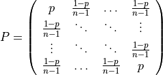
$P = \left(\begin{array}{cccc} p & \frac{1-p}{n-1} & \ldots & \frac{1-p}{n-1}\\ \frac{1-p}{n-1} & \ddots & \ddots & \vdots\\ \vdots & \ddots & \ddots & \frac{1-p}{n-1}\\ \frac{1-p}{n-1} & \ldots & \frac{1-p}{n-1} & p \end{array}\right)$

where $0\leqslant p < 1$ is a parameter.

Parameters:

n (int) – order of the kernel, number of states
p (float) – number in the interval [0, 1[
return_pinv (bool) – indicates if the invariant distribution is returned

Returns:

kernel (2d-array of shape (n, n)) – transition kernel (P) above
pinv ((1d-array of shape (n,)) – invariant distibution of the kernel, that is
- [1/n, … , 1/n]
returned if return_pinv=True

markovChain.mc_kernel2(n, p, return_pinv=False)

Sets the following transition kernel of order n for a Markov chain:

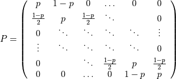
$P = \left(\begin{array}{cccccc} p & 1-p & 0 & \ldots & 0 & 0\\ \frac{1-p}{2} & p & \frac{1-p}{2} & \ddots & & 0\\ 0 & \ddots & \ddots & \ddots & \ddots & \vdots\\ \vdots & \ddots & \ddots & \ddots & \ddots & 0\\ 0 & & \ddots & \frac{1-p}{2} & p & \frac{1-p}{2}\\ 0 & 0 & \ldots & 0 & 1-p & p \end{array}\right)$

where $0\leqslant p < 1$ is a parameter.

Parameters:

n (int) – order of the kernel, number of states
p (float) – number in the interval [0, 1[
return_pinv (bool) – indicates if the invariant distribution is returned

Returns:

kernel (2d-array of shape (n, n)) – transition kernel (P) above
pinv ((1d-array of shape (n,)) – invariant distibution of the kernel, that is
- [1/(2(n-1)), 1/(n-1), … , 1/(n-1), 1/(2(n-1))]
returned if return_pinv=True

markovChain.mc_kernel3(n, p, q, return_pinv=False)

Sets the following transition kernel of order n for a Markov chain:

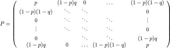
$P = \left(\begin{array}{ccccc} p & (1-p)q & 0 & \ldots & (1-p)(1-q)\\ (1-p)(1-q) & \ddots & \ddots & & 0\\ 0 & \ddots & \ddots & \ddots & \vdots\\ \vdots & \ddots & \ddots & \ddots & 0\\ 0 & & \ddots & \ddots & (1-p)q\\ (1-p)q & 0 & \ldots & (1-p)(1-q) & p \end{array}\right)$

where $0\leqslant p < 1$ and $0\leqslant q \leqslant 1$ are two parameters.

Parameters:

n (int) – order of the kernel, number of states
p (float) – number in the interval [0, 1[
q (float) – number in the interval [0, 1]
return_pinv (bool) – indicates if the invariant distribution is returned

Returns:

kernel (2d-array of shape (n, n)) – transition kernel (P) above
pinv ((1d-array of shape (n,)) – invariant distibution of the kernel, that is
- [1/n, … , 1/n]
returned if return_pinv=True

markovChain.mc_kernel4(n, p, q, return_pinv=False)

Sets the following transition kernel of order n for a Markov chain:

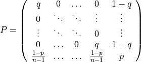
$P = \left(\begin{array}{ccccc} q & 0 & \ldots & 0 & 1-q\\ 0 & \ddots & \ddots & \vdots & \vdots\\ \vdots & \ddots & \ddots & 0 & \vdots\\ 0 & \ldots & 0 & q & 1-q\\ \frac{1-p}{n-1} & \ldots & \ldots &\frac{1-p}{n-1} & p \end{array}\right)$

where $0\leqslant p, q < 1$ are two parameters.

Parameters:

n (int) – order of the kernel, number of states
p (float) – number in the interval [0, 1[
q (float) – number in the interval [0, 1[
return_pinv (bool) – indicates if the invariant distribution is returned

Returns:

kernel (2d-array of shape (n, n)) – transition kernel (P) above
pinv ((1d-array of shape (n,)) – invariant distibution of the kernel, that is
- 1/(2-p-q) * [(1-p)/(n-1), … , (1-p)/(n-1), 1-q]
returned if return_pinv=True

markovChain.simulate_mc(kernel, nsteps, categVal=None, data_ind=None, data_val=None, pstep0=None, pinv=None, kernel_rev=None, kernel_pow=None, nreal=1, logger=None)

Generates (conditional) Markov chains for a given kernel.

Parameters:

kernel (2d-array of shape (n, n)) –
transition kernel of a Markov chain on a set of states $S=\{0, \ldots, n-1\}$ ; the element at row i and column j is the probability to have the state of index j at the next step given the state i at the current step, i.e.
- $kernel[i][j] = P(X_{k+1}=j\ \vert\ X_{k}=i)$
where the sequence of random variables $(X_k)$ is a Markov chain on S defined by the kernel kernel.

In particular, every element of kernel is positive or zero, and its rows sum to one.
nsteps (int) – length of each generated chain, number of time steps
categVal (1d-array of shape (n,), optional) – values of categories (one value for each state 0, …, n-1); by default (None) : categVal is set to [0, …, n-1]
data_ind (sequence, optional) – index (time step) of conditioning locations; each index should be in {0, 1, …, nsteps-1}
data_val (sequence, optional) – values at conditioning locations (same length as data_ind); each value should be in categVal
pstep0 (1d-array of shape (n,), optional) – distribution for step 0 of the chain, for unconditional simulation (used only if data_ind=None and data_val=None) by default (None): pinv is used (see below)
pinv (1d-array of shape (n,), optional) – invariant distribution of the Markov chain; by default (None): pinv is automatically computed
kernel_rev (2d-array of shape (n, n), optional) – reverse transition kernel of the Markov chain; by default (None): kernel_rev is automatically computed; note: only used for conditional simulation
kernel_pow (3d-array of shape (m, n, n), optional) –
pre-computed kernel raised to power 0, 1, …, m-1:
- $kernel\_pow[k] = kernel^k$
note: only used for conditional simulation
nreal (int, default: 1) – number of realization(s), number of generated chain(s)
logger (logging.Logger, optional) – logger (see package logging) if specified, messages are written via logger (no print)

Returns:

x – generated Markov chain (conditional to data_ind, data_val if present), x[i] is the i-th realization

Return type:

3d-array of shape (nreal, nsteps)

multiGaussian

Module for multi-Gaussian simulation and estimation in 1D, 2D and 3D, based on functions in other geone modules (wrapper).

exception multiGaussian.MultiGaussianError: Custom exception related to multiGaussian module.

multiGaussian.multiGaussianRun(cov_model, dimension, spacing=None, origin=None, mode='simulation', algo='fft', output_mode='img', retrieve_warnings=False, verbose=2, use_multiprocessing=False, logger=None, **kwargs)

Runs multi-Gaussian simulation or estimation.

Wrapper of other functions, the space dimension (1, 2, or 3) is detected (from the parameter dimension), and the method is selected according to the parameters mode and algo. Moreover, the type of output can be specified (parameter output_mode).

Parameters:

cov_model (geone.covModel.CovModel<d>D) – covariance model in 1D or 2D or 3D
dimension ([sequence of] int(s)) –
number of cells along each axis, for simulation in:
- 1D: dimension=nx
- 2D: dimension=(nx, ny)
- 3D: dimension=(nx, ny, nz)
note : this parameter determines the space dimension (1, 2, or 3)
spacing ([sequence of] float(s), optional) –
cell size along each axis, for simulation in:
- 1D: spacing=sx
- 2D: spacing=(sx, sy)
- 3D: spacing=(sx, sy, sz)
by default (None): 1.0 along each axis
origin ([sequence of] float(s), optional) –
origin of the grid (“corner of the first cell”), for simulation in:
- 1D: origin=ox
- 2D: origin=(ox, oy)
- 3D: origin=(ox, oy, oz)
by default (None): 0.0 along each axis
mode (str {'simulation', 'estimation'}, default: 'simulation') –
mode of computation:
- mode=’simulation’: generates multi-Gaussian simulations
- mode=’estimation’: computes multi-Gaussian estimation (and st. dev.)
algo (str {'fft', 'classic', 'classic_old'}, default: 'fft') –
defines the algorithm used:
- algo=’fft’: algorithm based on circulant embedding and FFT, function called for <d>D (d = 1, 2, or 3):
  - ’geone.grf.grf<d>D’, if mode=’simulation’
  - ’geone.grf.krige<d>D’, if mode=’estimation’
- algo=’classic’: “classic” algorithm, based on the resolution of kriging system considering points in a search ellipsoid, function called:
  - ’geone.geoscalassicinterface.simulate’, if mode=’simulation’
  - ’geone.geoscalassicinterface.estimate’, if mode=’estimation’
- algo=’classic_old’: “classic” algorithm (old version), based on the resolution of kriging system considering points in a search ellipsoid, function called for <d>D (d = 1, 2, or 3):
  - ’geone.geoscalassicinterface.simulate<d>D’, if mode=’simulation’
  - ’geone.geoscalassicinterface.estimate<d>D’, if mode=’estimation’
output_mode (str {'array', 'img'}, default: 'img') – defines the type of output returned (see below)
retrieve_warnings (bool, default: False) – indicates if the warnings encountered during the run are retrieved in output (True) or not (False) (see below)
verbose (int, default: 2) – verbose mode, higher implies more printing (info)
use_multiprocessing (bool, default: False) – indicates if multiprocessing is used in the case: algo=’classic_old’, mode=’simulation’); if use_multiprocessing=True, the function geone.geoscalassicinterface.simulate<d>D_mp is used instead of geone.geoscalassicinterface.simulate<d>D; in other cases use_multiprocessing is ignored
logger (logging.Logger, optional) – logger (see package logging) if specified, messages are written via logger (no print)
kwargs (dict) – keyword arguments (additional parameters) to be passed to the function that is called (according to algo and space dimension); note: argument mask can also be used with algo=’fft’; in this case the mask is applied afterward

Returns:

output (ndarray or geone.img.Img) –
- if output_mode=’array’: output is a ndarray of shape
  - for 1D:
    
    (1, nx) if mode=’estimation’ with kriging estimate only
    
    (2, nx) if mode=’estimation’ with kriging estimate and st. dev.
    
    (nreal, nx) if mode=’simulation’
  - for 2D:
    
    (1, ny, nx) if mode=’estimation’ with kriging estimate only
    
    (2, ny, nx) if mode=’estimation’ with kriging estimate and st. dev.
    
    (nreal, ny, nx) if mode=’simulation’
  - for 3D:
    
    (1, nz, ny, nx) if mode=’estimation’ with krig. est. only
    
    (2, nz, ny, nx) if mode=’estimation’ with krig. est. and st. dev.
    
    (nreal, nz, ny, nx) if mode=’simulation’
- if output_mode=’img’: output is an instance of geone.img.Img an image with output.nv variables:
  - output.nv=1 if mode=’estimation’ with kriging estimate only
  - output.nv=2 if mode=’estimation’ with krig. est. and st. dev.
  - output.nv=nreal if mode=’simulation’
warnings (list of strs, optional) – list of distinct warnings encountered (can be empty) during the run (no warning (empty list) if algo=’fft’); returned if retrieve_warnings=True

pgs

Module for plurig-Gaussian simulations in 1D, 2D and 3D.

exception pgs.PgsError: Custom exception related to pgs module.

pgs.pluriGaussianSim(cov_model_T1, cov_model_T2, flag_value, dimension, spacing=None, origin=None, x=None, v=None, algo_T1='fft', params_T1={}, algo_T2='fft', params_T2={}, accept_init=0.25, accept_pow=2.0, mh_iter_min=100, mh_iter_max=200, ntry_max=1, retrieve_real_anyway=False, nreal=1, full_output=True, verbose=1, logger=None)

Generates (conditional) pluri-Gaussian simulations.

The simulated variable Z at a point x is defined as

Z(x) = flag_value(T1(x), T2(x))

where

T1, T2 are two multi-Gaussian random fields (latent fields)
flag_value is a function of two variables defining the final value (given as a “flag”)

Z and T1, T2 are fields in 1D, 2D or 3D.

Parameters:

cov_model_T1 (geone.covModel.CovModel<d>D) – covariance model for T1, in 1D or 2D or 3D (same space dimension for T1 and T2); note: if algo_T1=’deterministic’, cov_model_T1 can be None (unused)
cov_model_T2 (geone.covModel.CovModel<d>D) – covariance model for T2, in 1D or 2D or 3D (same space dimension for T1 and T2); note: if algo_T2=’deterministic’, cov_model_T2 can be None (unused)
flag_value (function (callable)) – function of tow arguments (xi, yi) that returns the “flag_value” at location (xi, yi)
dimension ([sequence of] int(s)) –
number of cells along each axis, for simulation in:
- 1D: dimension=nx
- 2D: dimension=(nx, ny)
- 3D: dimension=(nx, ny, nz)
spacing ([sequence of] float(s), optional) –
cell size along each axis, for simulation in:
- 1D: spacing=sx
- 2D: spacing=(sx, sy)
- 3D: spacing=(sx, sy, sz)
by default (None): 1.0 along each axis
origin ([sequence of] float(s), optional) –
origin of the grid (“corner of the first cell”), for simulation in:
- 1D: origin=ox
- 2D: origin=(ox, oy)
- 3D: origin=(ox, oy, oz)
by default (None): 0.0 along each axis
x (array-like of floats, optional) –
data points locations (float coordinates), for simulation in:
- 1D: 1D array-like of floats
- 2D: 2D array-like of floats of shape (n, 2)
- 3D: 2D array-like of floats of shape (n, 3)
note: if one point (n=1), a float in 1D, a 1D array of shape (2,) in 2D, a 1D array of shape (3,) in 3D, is accepted
v (1D array-like of floats, optional) – data values at x (v[i] is the data value at x[i])
algo_T1 (str {'fft', 'classic', 'deterministic'}, default: 'fft') –
defines the algorithm used for T1:
- ’fft’: algorithm based on circulant embedding and FFT, function called for <d>D (d = 1, 2, or 3): ‘geone.grf.grf<d>D’
- ’classic’: “classic” algorithm, based on the resolution of kriging system considered points in a search ellipsoid, function called for <d>D (d = 1, 2, or 3): ‘geone.geoscalassicinterface.simulate<d>D’
- ’deterministic’: use a deterministic field, given by param_T1[‘mean’]
algo_T2 (str {'fft', 'classic', 'deterministic'}, default: 'fft') – defines the algorithm used for T2 (see algo_T1 for detail)
params_T1 (dict) – keyword arguments (additional parameters) to be passed to the function that is called (according to algo_T1 and space dimension) for simulation of T1
params_T2 (dict) – keyword arguments (additional parameters) to be passed to the function that is called (according to algo_T2 and space dimension) for simulation of T2
accept_init (float, default: 0.25) – initial acceptation probability (see parameters mh_iter_min, mh_iter_max)
accept_pow (float, default: 2.0) – power for computing acceptation probability (see parameters mh_iter_min, mh_iter_max)
mh_iter_min (int, default: 100) – see parameter mh_iter_max
mh_iter_max (int, default: 200) –
mh_iter_min and mh_iter_max are the number of iterations (min and max) for Metropolis-Hasting algorithm (for conditional simulation) when updating T1 and T2 at conditioning locations at iteration nit (in 0, …, mh_iter_max-1):
- if nit < mh_iter_min: for any k:
  - simulate new candidate at x[k]: (T1(x[k]), T2(x[k]))
  - if flag_value(T1(x[k]), T2(x[k])=v[k] (conditioning ok): accept the new candidate
  - else (conditioning not ok): accept the new candidate with probability
    
    p = accept_init * (1 - 1/mh_iter_min)**accept_pow
- if nit >= mh_iter_min:
  - if conditioning ok at every x[k]: stop and exit the loop,
  - else: for any k:
    
    if conditioning ok at x[k]: skip
    
    else:
    
    simulate new candidate at x[k]: (T1(x[k]), T2(x[k]))
    
    if flag_value(T1(x[k]), T2(x[k])=v[k] (conditioning ok): accept the new candidate
    
    else (conditioning not ok): reject the new candidate
ntry_max (int, default: 1) – number of trial(s) per realization before giving up if something goes wrong
retrieve_real_anyway (bool, default: False) –
if after ntry_max trial(s) a conditioning data is not honoured, then the realization is:
- retrieved, if retrieve_real_anyway=True
- not retrieved (missing realization), if retrieve_real_anyway=False
nreal (int, default: 1) – number of realization(s)
full_output (bool, default: True) –
- if True: simulation(s) of Z, T1, T2, and n_cond_ok are retrieved in output
- if False: simulation(s) of Z only is retrieved in output
verbose (int, default: 1) – verbose mode, higher implies more printing (info)
logger (logging.Logger, optional) – logger (see package logging) if specified, messages are written via logger (no print)

Returns:

Z (ndarray) – array of shape
- for 1D: (nreal, nx)
- for 2D: (nreal, ny, nx)
- for 3D: (nreal, nz, ny, nx)
Z[k] is the k-th realization of Z
T1 (ndarray, optional) – array of shape
- for 1D: (nreal, nx)
- for 2D: (nreal, ny, nx)
- for 3D: (nreal, nz, ny, nx)
T1[k] is the k-th realization of T1; returned if full_output=True
T2 (ndarray, optional) – array of shape
- for 1D: (nreal, nx)
- for 2D: (nreal, ny, nx)
- for 3D: (nreal, nz, ny, nx)
T2[k] is the k-th realization of T2; returned if full_output=True
n_cond_ok (list of 1D array) – list of length nreal
- n_cond_ok[k]: 1D array of ints
  number of conditioning locations honoured at each iteration of the Metropolis-Hasting algorithm for the k-th realization, in particular len(n_cond_ok[k]) is the number of iteration done, n_cond_ok[k][-1] is the number of conditioning locations honoured at the end;
returned if full_output=True

pgs.pluriGaussianSim_unconditional(cov_model_T1, cov_model_T2, flag_value, dimension, spacing=None, origin=None, algo_T1='fft', params_T1={}, algo_T2='fft', params_T2={}, nreal=1, full_output=True, verbose=1, logger=None)

Generates unconditional pluri-Gaussian simulations.

The simulated variable Z at a point x is defined as

Z(x) = flag_value(T1(x), T2(x))

where

T1, T2 are two multi-Gaussian random fields (latent fields)
flag_value is a function of two variables defining the final value (given as a “flag”)

Z and T1, T2 are fields in 1D, 2D or 3D.

Parameters:

cov_model_T1 (geone.covModel.CovModel<d>D) – covariance model for T1, in 1D or 2D or 3D (same space dimension for T1 and T2); note: if algo_T1=’deterministic’, cov_model_T1 can be None (unused)
cov_model_T2 (geone.covModel.CovModel<d>D) – covariance model for T2, in 1D or 2D or 3D (same space dimension for T1 and T2); note: if algo_T2=’deterministic’, cov_model_T2 can be None (unused)
flag_value (function (callable)) – function of tow arguments (xi, yi) that returns the “flag_value” at location (xi, yi)
dimension ([sequence of] int(s)) –
number of cells along each axis, for simulation in:
- 1D: dimension=nx
- 2D: dimension=(nx, ny)
- 3D: dimension=(nx, ny, nz)
spacing ([sequence of] float(s), optional) –
cell size along each axis, for simulation in:
- 1D: spacing=sx
- 2D: spacing=(sx, sy)
- 3D: spacing=(sx, sy, sz)
by default (None): 1.0 along each axis
origin ([sequence of] float(s), optional) –
origin of the grid (“corner of the first cell”), for simulation in:
- 1D: origin=ox
- 2D: origin=(ox, oy)
- 3D: origin=(ox, oy, oz)
by default (None): 0.0 along each axis
algo_T1 (str {'fft', 'classic', 'deterministic'}, default: 'fft') –
defines the algorithm used for T1:
- ’fft’: algorithm based on circulant embedding and FFT, function called for <d>D (d = 1, 2, or 3): ‘geone.grf.grf<d>D’
- ’classic’: “classic” algorithm, based on the resolution of kriging system considered points in a search ellipsoid, function called for <d>D (d = 1, 2, or 3): ‘geone.geoscalassicinterface.simulate<d>D’
- ’deterministic’: use a deterministic field, given by param_T1[‘mean’]
algo_T2 (str {'fft', 'classic', 'deterministic'}, default: 'fft') – defines the algorithm used for T2 (see algo_T1 for detail)
params_T1 (dict) – keyword arguments (additional parameters) to be passed to the function that is called (according to algo_T1 and space dimension) for simulation of T1
params_T2 (dict) – keyword arguments (additional parameters) to be passed to the function that is called (according to algo_T2 and space dimension) for simulation of T2
nreal (int, default: 1) – number of realization(s)
full_output (bool, default: True) –
- if True: simulation(s) of Z, T1, and T2 are retrieved in output
- if False: simulation(s) of Z only is retrieved in output
verbose (int, default: 1) – verbose mode, higher implies more printing (info)
logger (logging.Logger, optional) – logger (see package logging) if specified, messages are written via logger (no print)

Returns:

Z (ndarray) – array of shape
- for 1D: (nreal, nx)
- for 2D: (nreal, ny, nx)
- for 3D: (nreal, nz, ny, nx)
Z[k] is the k-th realization of Z
T1 (ndarray, optional) – array of shape
- for 1D: (nreal, nx)
- for 2D: (nreal, ny, nx)
- for 3D: (nreal, nz, ny, nx)
T1[k] is the k-th realization of T1; returned if full_output=True
T2 (ndarray, optional) – array of shape
- for 1D: (nreal, nx)
- for 2D: (nreal, ny, nx)
- for 3D: (nreal, nz, ny, nx)
T2[k] is the k-th realization of T2; returned if full_output=True

srf

Module for the generation of random fields based on substitution random function (SRF). Random fields in 1D, 2D, 3D.

References

1. Straubhaar, P. Renard (2024), Exploring substitution random functions composed of stationary multi-Gaussian processes. Stochastic Environmental Research and Risk Assessment, doi:10.1007/s00477-024-02662-x
1. Lantuéjoul (2002) Geostatistical Simulation, Models and Algorithms. Springer Verlag, Berlin, 256 p.

class srf.Distrib(pdf=None, cdf=None, ppf=None): Class defining a distribution by a pdf, cdf, and ppf.

exception srf.SrfError: Custom exception related to srf module.

srf.compute_distrib_Z_given_Y_of_mean_T(z, cov_model_Y, mean_Y=0.0, y_mean_T=0.0, cov_T_0=1.0, fstd=4.5, nint=2001, assume_sorted=False)

Computes the distribution of Z given Y(mean(T)), for a SRF Z = Y(T).

With a SRF Z = Y(T), compute the pdf, cdf and ppf (inverse cdf) of Z given Y(mean(T))=y_mean_T (applicable for a (large) ensemble of realizations).

The cdf is given by the equation (26) in the reference below. This equation requires expectations wrt. $\mathcal{N}(0, c\_T\_0)$ , which are approximated using nint values in the interval $\pm fstd \cdot \sqrt{c\_T\_0}$ .

Parameters:

z (1d-array of floats) – values at which the conditional cdf and pdf are evaluated before interpolation, e.g numpy.linspace(z_min, z_max, n) with given z_min, z_max, and n
cov_model_Y (geone.covModel.CovModel1D) – covariance model for Y (coding process), in 1D
mean_Y (float, default: 0.0) – mean of Y
y_mean_T (float, default: 0.0) – imposed value for Y(mean(T))
cov_T_0 (float, default: 1.0) – covariance model of T (latent field, directing function) evaluated at 0
fstd (float, default: 4.5) – positive value used for computing approximation (see above)
nint (int, defualt: 2001) – positive integer used for computing approximation (see above)
assume_sorted (bool, default: False) – if True: z has to be an array of monotonically increasing values

Returns:

distrib – distribution, where each attribute is a function (obtained by interpolation of its approximated evaluation at z):

distrib.pdf: (func) pdf f_{Z|Y(mean(T))=y_mean_T}
distrib.cdf: (func) cdf F_{Z|Y(mean(T))=y_mean_T}
distrib.ppf: (func) inverse cdf

Return type:

Distrib

References

1. Straubhaar, P. Renard (2024), Exploring substitution random functions composed of stationary multi-Gaussian processes. Stochastic Environmental Research and Risk Assessment, doi:10.1007/s00477-024-02662-x

srf.srf_bimg_mg(cov_model_T1, cov_model_T2, cov_model_Y, dimension, spacing=None, origin=None, spacing_Y=(0.001, 0.001), x=None, v=None, t=None, yt=None, vmin=None, vmax=None, algo_T1='fft', params_T1=None, algo_T2='fft', params_T2=None, algo_Y='fft', params_Y=None, mh_iter=100, ntry_max=1, nreal=1, full_output=True, verbose=1, logger=None)

Substitution Random Function (SRF) - multi-Gaussian + multi-Gaussian.

This function allows to generate continuous random fields in 1D, 2D, 3D, based on a SRF Z defined as

Z(x) = Y(T1(x), T2(x))

where

T1, T1 are the directing functions (independent), two multi-Gaussian random fields (latent fields)
Y is the coding process, a 2D multi-Gaussian random field

Z and T1, T2 are fields in 1D, 2D or 3D.

Notes

The module multiGaussian is used for the multi-Gaussian fields T1, T2 and Y.

Parameters:

cov_model_T1 (geone.covModel.CovModel<d>D) – covariance model for T1, in 1D or 2D or 3D; note: can be set to None; in this case, algo_T1=’deterministic’ is requiered and params_T1[‘mean’] defines the field T1
cov_model_T2 (geone.covModel.CovModel<d>D) – covariance model for T2, in 1D or 2D or 3D note: can be set to None; in this case, algo_T2=’deterministic’ is requiered and params_T2[‘mean’] defines the field T2
cov_model_Y (geone.covModel.CovModel2D) – covariance model for Y, in 2D
dimension ([sequence of] int(s)) –
number of cells along each axis, for simulation in:
- 1D: dimension=nx
- 2D: dimension=(nx, ny)
- 3D: dimension=(nx, ny, nz)
spacing ([sequence of] float(s), optional) –
cell size along each axis, for simulation in:
- 1D: spacing=sx
- 2D: spacing=(sx, sy)
- 3D: spacing=(sx, sy, sz)
by default (None): 1.0 along each axis
origin ([sequence of] float(s), optional) –
origin of the grid (“corner of the first cell”), for simulation in:
- 1D: origin=ox
- 2D: origin=(ox, oy)
- 3D: origin=(ox, oy, oz)
by default (None): 0.0 along each axis
spacing_Y (sequence of 2 floats, default: (0.001, 0.001)) – two positive values, resolution of the 2D Y field, along the two dimensions (corresponding to T1 and T2), spacing between two adjacent cells in the two directions
x (array-like of floats, optional) –
data points locations (float coordinates), for simulation in:
- 1D: 1D array-like of floats
- 2D: 2D array-like of floats of shape (m, 2)
- 3D: 2D array-like of floats of shape (m, 3)
note: if one point (m=1), a float in 1D, a 1D array of shape (2,) in 2D, a 1D array of shape (3,) in 3D, is accepted
v (1d-array-like of floats, optional) – data values at x (v[i] is the data value at x[i])
t (2d-array of floats or sequence of 2 floats, optional) – values of (T1, T2) considered as conditioning point for Y(T) (additional constraint)m each row corresponding to one point; note: if only one point, a sequence of 2 floats is accepted
yt (1d-array-like of floats, or float, optional) – value of Y at the conditioning point t
vmin (float, optional) – minimal value for Z (or Y); simulation are rejected if not honoured
vmax (float, optional) – maximal value for Z (or Y); simulation are rejected if not honoured
algo_T1 (str) –
defines the algorithm used for generating multi-Gaussian field T1:
- ’fft’ or ‘FFT’ (default): based on circulant embedding and FFT, function called for <d>D (d = 1, 2, or 3): geone.grf.grf<d>D
- ’classic’ or ‘CLASSIC’: classic algorithm, based on the resolution of kriging system considered points in a search ellipsoid, function called for <d>D (d = 1, 2, or 3): geone.geoscalassicinterface.simulate<d>D
- ’deterministic’ or ‘DETERMINISTIC’: use a deterministic field defined by params_T1[‘mean’]
params_T1 (dict, optional) – keyword arguments (additional parameters) to be passed to the function corresponding to what is specified by the argument algo_T1 (see the corresponding function for its keyword arguments), in particular the key ‘mean’ can be specified (set to value 0 if not specified)
algo_T2 (str) –
defines the algorithm used for generating multi-Gaussian field T2:
- ’fft’ or ‘FFT’ (default): based on circulant embedding and FFT, function called for <d>D (d = 1, 2, or 3): geone.grf.grf<d>D
- ’classic’ or ‘CLASSIC’: classic algorithm, based on the resolution of kriging system considered points in a search ellipsoid, function called for <d>D (d = 1, 2, or 3): geone.geoscalassicinterface.simulate<d>D
- ’deterministic’ or ‘DETERMINISTIC’: use a deterministic field defined by params_T2[‘mean’]
params_T2 (dict, optional) – keyword arguments (additional parameters) to be passed to the function corresponding to what is specified by the argument algo_T2 (see the corresponding function for its keyword arguments), in particular the key ‘mean’ can be specified (set to value 0 if not specified)
algo_Y (str) –
defines the algorithm used for generating 2D multi-Gaussian field Y:
- ’fft’ or ‘FFT’ (default): based on circulant embedding and FFT, function called: geone.grf.grf2D()
- ’classic’ or ‘CLASSIC’: classic algorithm, based on the resolution of kriging system considered points in a search ellipsoid, function called: geone.geoscalassicinterface.simulate()
params_Y (dict, optional) – keyword arguments (additional parameters) to be passed to the function corresponding to what is specified by the argument algo_Y (see the corresponding function for its keyword arguments), in particular the key ‘mean’ can be specified (if not specified, set to the mean value of v if v is not None, set to 0 otherwise)
mh_iter (int, default: 100) – number of iteration for Metropolis-Hasting algorithm, for conditional simulation only; note: used only if x or t is not None
ntry_max (int, default: 1) – number of tries per realization before giving up if something goes wrong
nreal (int, default: 1) – number of realization(s)
full_output (bool, default: True) –
- if True: simulation(s) of Z, T1, T2, and Y are retrieved in output
- if False: simulation(s) of Z only is retrieved in output
verbose (int, default: 1) – verbose mode, integer >=0, higher implies more display
logger (logging.Logger, optional) – logger (see package logging) if specified, messages are written via logger (no print)

Returns:

Z (nd-array) – all realizations, Z[k] is the k-th realization:
- for 1D: Z of shape (nreal, nx), where nx = dimension
- for 2D: Z of shape (nreal, ny, nx), where nx, ny = dimension
- for 3D: Z of shape (nreal, nz, ny, nx), where nx, ny, nz = dimension
T1 (nd-array) – latent fields of all realizations, T1[k] for the k-th realization:
- for 1D: T1 of shape (nreal, nx), where nx = dimension
- for 2D: T1 of shape (nreal, ny, nx), where nx, ny = dimension
- for 3D: T1 of shape (nreal, nz, ny, nx), where nx, ny, nz = dimension
returned if full_output=True
T2 (nd-array) – latent fields of all realizations, T2[k] for the k-th realization:
- for 1D: T2 of shape (nreal, nx), where nx = dimension
- for 2D: T2 of shape (nreal, ny, nx), where nx, ny = dimension
- for 3D: T2 of shape (nreal, nz, ny, nx), where nx, ny, nz = dimension
returned if full_output=True
Y (list of length nreal) – 2D random fields of all realizations, Y[k] is a list of length 4 for the k-th realization:
- Y[k][0]: 1d-array of shape (2,): (Y_nx, Y_ny)
- Y[k][1]: 1d-array of shape (2,): (Y_sx, Y_sy)
- Y[k][2]: 1d-array of shape (2,): (Y_ox, Y_oy)
- Y[k][3]: 2d-array of shape (Y_ny, Y_nx): values of Y[k]
returned if full_output=True

srf.srf_mg_mc(cov_model_T, kernel_Y, dimension, spacing=None, origin=None, spacing_Y=0.001, categVal=None, x=None, v=None, t=None, yt=None, algo_T='fft', params_T=None, mh_iter=100, ntry_max=1, nreal=1, full_output=True, verbose=1, logger=None)

Substitution Random Function (SRF) - multi-Gaussian + Markov chain (on finite set).

This function allows to generate categorical random fields in 1D, 2D, 3D, based on a SRF Z defined as

Z(x) = Y(T(x))

where

T is the directing function, a multi-Gaussian random field (latent field)
Y is the coding process, a Markov chain on finite sets (of categories) (1D)

Z and T are fields in 1D, 2D or 3D.

Notes

The module multiGaussian is used for the multi-Gaussian field T, and the module markovChain is used for the markov chain Y.

Parameters:

cov_model_T (geone.covModel.CovModel<d>D) – covariance model for T, in 1D or 2D or 3D
kernel_Y (2d-array of shape (n, n)) –
transition kernel for Y of a Markov chain on a set of states $S=\{0, \ldots, n-1\}$ , where n is the number of categories (states); the element at row i and column j is the probability to have the state of index j at the next step given the state i at the current step, i.e.
- $kernel[i][j] = P(Y_{k+1}=j\ \vert\ Y_{k}=i)$
where the sequence of random variables $(Y_k)$ is a Markov chain on S defined by the kernel kernel.

In particular, every element of kernel is positive or zero, and its rows sum to one.
dimension ([sequence of] int(s)) –
number of cells along each axis, for simulation in:
- 1D: dimension=nx
- 2D: dimension=(nx, ny)
- 3D: dimension=(nx, ny, nz)
spacing ([sequence of] float(s), optional) –
cell size along each axis, for simulation in:
- 1D: spacing=sx
- 2D: spacing=(sx, sy)
- 3D: spacing=(sx, sy, sz)
by default (None): 1.0 along each axis
origin ([sequence of] float(s), optional) –
origin of the grid (“corner of the first cell”), for simulation in:
- 1D: origin=ox
- 2D: origin=(ox, oy)
- 3D: origin=(ox, oy, oz)
by default (None): 0.0 along each axis
spacing_Y (float, default: 0.001) – positive value, resolution of the Y process, spacing along abscissa between two steps in the Markov chain Y (btw. two adjacent cell in 1D-grid for Y)
categVal (1d-array of shape (n,), optional) – values of categories (one value for each state 0, …, n-1); by default (None) : categVal is set to [0, …, n-1]
x (array-like of floats, optional) –
data points locations (float coordinates), for simulation in:
- 1D: 1D array-like of floats
- 2D: 2D array-like of floats of shape (m, 2)
- 3D: 2D array-like of floats of shape (m, 3)
note: if one point (m=1), a float in 1D, a 1D array of shape (2,) in 2D, a 1D array of shape (3,) in 3D, is accepted
v (1d-array-like of floats, optional) – data values at x (v[i] is the data value at x[i])
t (1d-array-like of floats, or float, optional) – values of T considered as conditioning point for Y(T) (additional constraint)
yt (1d-array-like of floats, or float, optional) – value of Y at the conditioning point t (same length as t)
algo_T (str) –
defines the algorithm used for generating multi-Gaussian field T:
- ’fft’ or ‘FFT’ (default): based on circulant embedding and FFT, function called for <d>D (d = 1, 2, or 3): geone.grf.grf<d>D
- ’classic’ or ‘CLASSIC’: classic algorithm, based on the resolution of kriging system considered points in a search ellipsoid, function called for <d>D (d = 1, 2, or 3): geone.geoscalassicinterface.simulate<d>D
params_T (dict, optional) – keyword arguments (additional parameters) to be passed to the function corresponding to what is specified by the argument algo_T (see the corresponding function for its keyword arguments), in particular the key ‘mean’ can be specified (set to value 0 if not specified)
mh_iter (int, default: 100) – number of iteration for Metropolis-Hasting algorithm, for conditional simulation only; note: used only if x or t is not None
ntry_max (int, default: 1) – number of tries per realization before giving up if something goes wrong
nreal (int, default: 1) – number of realization(s)
full_output (bool, default: True) –
- if True: simulation(s) of Z, T, and Y are retrieved in output
- if False: simulation(s) of Z only is retrieved in output
verbose (int, default: 1) – verbose mode, integer >=0, higher implies more display
logger (logging.Logger, optional) – logger (see package logging) if specified, messages are written via logger (no print)

Returns:

Z (nd-array) – all realizations, Z[k] is the k-th realization:
- for 1D: Z of shape (nreal, nx), where nx = dimension
- for 2D: Z of shape (nreal, ny, nx), where nx, ny = dimension
- for 3D: Z of shape (nreal, nz, ny, nx), where nx, ny, nz = dimension
T (nd-array) – latent fields of all realizations, T[k] for the k-th realization:
- for 1D: T of shape (nreal, nx), where nx = dimension
- for 2D: T of shape (nreal, ny, nx), where nx, ny = dimension
- for 3D: T of shape (nreal, nz, ny, nx), where nx, ny, nz = dimension
returned if full_output=True
Y (list of length nreal) – markov chains of all realizations, Y[k] is a list of length 4 for the k-th realization:
- Y[k][0]: int, Y_nt (number of cell along t-axis)
- Y[k][1]: float, Y_st (cell size along t-axis)
- Y[k][2]: float, Y_ot (origin)
- Y[k][3]: 1d-array of shape (Y_nt,), values of Y[k]
returned if full_output=True

srf.srf_mg_mg(cov_model_T, cov_model_Y, dimension, spacing=None, origin=None, spacing_Y=0.001, x=None, v=None, t=None, yt=None, vmin=None, vmax=None, algo_T='fft', params_T=None, algo_Y='fft', params_Y=None, target_distrib=None, initial_distrib=None, mh_iter=100, ntry_max=1, nreal=1, full_output=True, verbose=1, logger=None)

Substitution Random Function (SRF) - multi-Gaussian + multi-Gaussian.

This function allows to generate continuous random fields in 1D, 2D, 3D, based on a SRF Z defined as

Z(x) = Y(T(x))

where

T is the directing function, a multi-Gaussian random field (latent field)
Y is the coding process, a multi-Gaussian random process (1D)

Z and T are fields in 1D, 2D or 3D.

Notes

The module multiGaussian is used for the multi-Gaussian fields T and Y.

Parameters:

cov_model_T (geone.covModel.CovModel<d>D) – covariance model for T, in 1D or 2D or 3D
cov_model_Y (geone.covModel.CovModel1D) – covariance model for Y, in 1D
dimension ([sequence of] int(s)) –
number of cells along each axis, for simulation in:
- 1D: dimension=nx
- 2D: dimension=(nx, ny)
- 3D: dimension=(nx, ny, nz)
spacing ([sequence of] float(s), optional) –
cell size along each axis, for simulation in:
- 1D: spacing=sx
- 2D: spacing=(sx, sy)
- 3D: spacing=(sx, sy, sz)
by default (None): 1.0 along each axis
origin ([sequence of] float(s), optional) –
origin of the grid (“corner of the first cell”), for simulation in:
- 1D: origin=ox
- 2D: origin=(ox, oy)
- 3D: origin=(ox, oy, oz)
by default (None): 0.0 along each axis
spacing_Y (float, default: 0.001) – positive value, resolution of the Y process, spacing along abscissa between two cells in the field Y (btw. two adjacent cell in 1D-grid for Y)
x (array-like of floats, optional) –
data points locations (float coordinates), for simulation in:
- 1D: 1D array-like of floats
- 2D: 2D array-like of floats of shape (m, 2)
- 3D: 2D array-like of floats of shape (m, 3)
note: if one point (m=1), a float in 1D, a 1D array of shape (2,) in 2D, a 1D array of shape (3,) in 3D, is accepted
v (1d-array-like of floats, optional) – data values at x (v[i] is the data value at x[i])
t (1d-array-like of floats, or float, optional) – values of T considered as conditioning point for Y(T) (additional constraint)
yt (1d-array-like of floats, or float, optional) – value of Y at the conditioning point t (same length as t)
vmin (float, optional) – minimal value for Z (or Y); simulation are rejected if not honoured
vmax (float, optional) – maximal value for Z (or Y); simulation are rejected if not honoured
algo_T (str) –
defines the algorithm used for generating multi-Gaussian field T:
- ’fft’ or ‘FFT’ (default): based on circulant embedding and FFT, function called for <d>D (d = 1, 2, or 3): geone.grf.grf<d>D
- ’classic’ or ‘CLASSIC’: classic algorithm, based on the resolution of kriging system considered points in a search ellipsoid, function called for <d>D (d = 1, 2, or 3): geone.geoscalassicinterface.simulate<d>D
params_T (dict, optional) – keyword arguments (additional parameters) to be passed to the function corresponding to what is specified by the argument algo_T (see the corresponding function for its keyword arguments), in particular the key ‘mean’ can be specified (set to value 0 if not specified)
algo_Y (str) –
defines the algorithm used for generating 1D multi-Gaussian field Y:
- ’fft’ or ‘FFT’ (default): based on circulant embedding and FFT, function called: geone.grf.grf1D()
- ’classic’ or ‘CLASSIC’: classic algorithm, based on the resolution of kriging system considered points in a search ellipsoid, function called: geone.geoscalassicinterface.simulate()
params_Y (dict, optional) – keyword arguments (additional parameters) to be passed to the function corresponding to what is specified by the argument algo_Y (see the corresponding function for its keyword arguments), in particular the key ‘mean’ can be specified (if not specified, set to the mean value of v if v is not None, set to 0 otherwise)
target_distrib (class) –
target distribution for the value of a single realization of Z, with attributes:
- target_distrib.cdf : (func) cdf
- target_distrib.ppf : (func) inverse cdf
See initial_distrib below.
initial_distrib (class) –
initial distribution for the value of a single realization of Z, with attributes:
- initial_distrib.cdf : (func) cdf
- initial_distrib.ppf : (func) inverse cdf
The procedure is the following:
1. conditioning data value v (if present) are transormed:
  - v_tilde = initial_distrib.ppf(target_distrib.cdf(v))
2. SRF realization of z_tilde (conditionally to v_tilde if present) is generated
3. back-transform is applied to obtain the final realization:
  - z = target_distrib.ppf(initial_distrib.cdf(z_tilde))
By default:
- target_distrib = None
- initial_distrib = None
- For unconditional case:
  - if target_distrib is None: no transformation is applied
  - otherwise (not None): transformation is applied (step 3. above)
- For conditional case:
  - if target_distrib is None: no transformation is applied
  - otherwise (not None): transformation is applied (steps 1 and 3. above); this requires that initial_distrib is specified (not None), or that t and yt are specified with the value “mean_T” given in t
The distribution initial_distrib is used when needed:
- as specified (if not None, be sure of what is given)
- computed automatically otherwise (if None): the distribution returned by the function compute_distrib_Z_given_Y_of_mean_T(), with the keyword arguments (only for unconditional case)
  - mean_Y : set to mean_Y (see above)
  - cov_T_0 : set to the covariance of T evaluated at 0 (cov_model_T.func()(0)[0])
  - y_mean_T: set to yt[i0], where t[i0]=mean_T (if exists, see t, yt above) or set to Y(mean(T)) computed after step 2 above (otherwise)
mh_iter (int, default: 100) – number of iteration for Metropolis-Hasting algorithm, for conditional simulation only; note: used only if x or t is not None
ntry_max (int, default: 1) – number of tries per realization before giving up if something goes wrong
nreal (int, default: 1) – number of realization(s)
full_output (bool, default: True) –
- if True: simulation(s) of Z, T, and Y are retrieved in output
- if False: simulation(s) of Z only is retrieved in output
verbose (int, default: 1) – verbose mode, integer >=0, higher implies more display
logger (logging.Logger, optional) – logger (see package logging) if specified, messages are written via logger (no print)

Returns:

Z (nd-array) – all realizations, Z[k] is the k-th realization:
- for 1D: Z of shape (nreal, nx), where nx = dimension
- for 2D: Z of shape (nreal, ny, nx), where nx, ny = dimension
- for 3D: Z of shape (nreal, nz, ny, nx), where nx, ny, nz = dimension
T (nd-array) – latent fields of all realizations, T[k] for the k-th realization:
- for 1D: T of shape (nreal, nx), where nx = dimension
- for 2D: T of shape (nreal, ny, nx), where nx, ny = dimension
- for 3D: T of shape (nreal, nz, ny, nx), where nx, ny, nz = dimension
returned if full_output=True
Y (list of length nreal) – 1D random fields of all realizations, Y[k] is a list of length 4 for the k-th realization:
- Y[k][0]: int, Y_nt (number of cell along t-axis)
- Y[k][1]: float, Y_st (cell size along t-axis)
- Y[k][2]: float, Y_ot (origin)
- Y[k][3]: 1d-array of shape (Y_nt,), values of Y[k]
returned if full_output=True

randProcess

Module for miscellaneous algorithms based on random processes.

exception randProcess.RandProcessError: Custom exception related to randProcess module.

randProcess.acceptRejectSampler(n, xmin, xmax, f, c=None, g=None, g_rvs=None, return_accept_ratio=False, max_trial=None, verbose=0, show_progress=None, opt_kwargs=None, logger=None)

Generates samples according to a given density function.

This function generates n points (which can be multi-variate) in a box-shape domain of lower bound(s) xmin and upper bound(s) xmax, according to a density proportional to the function f, based on the accept-reject algorithm.

Let g_rvs a function returning random variates sample(s) from an instrumental distribution with density proportional to g, and c a constant such that c*g(x) >= f(x) for any x (in [xmin, xmax[ (can be multi-dimensional), i.e. x[i] in [xmin[i], xmax[i][ for any i). Let fd (resp. gd) the density function proportional to f (resp. g); the alogrithm consists in the following steps to generate samples x ~ fd:

generate y ~ gd (using g_rvs)
generate u ~ Unif([0,1])
if u < f(y)/c*g(y), then accept x (reject x otherwise)

The default instrumental distribution (if both g and g_rvs set to None) is the uniform distribution (g=1). If the domain ([xmin, xmax[) is infinite, the instrumental distribution (g, and g_rvs) and c must be specified.

Parameters:

n (int) – number of sample points
xmin (float (or int), or array-like of shape(m,)) – lower bound of each coordinate (m is the space dimension); note: component(s) can be set to -np.inf
xmax (float (or int), or array-like of shape(m,)) – upper bound of each coordinate (m is the space dimension) note: component(s) can be set to np.inf
f (function (callable)) – function proportional to target density, f(x) returns the target density (times a constant) at x; with x array_like, the last axis of x denotes the components of the points where the function is evaluated
c (float (or int), optional) – constant such that (not checked)) c*g(x) >= f(x) for all x in [xmin, xmax[, with g(x)=1 if g is not specified (g=None); by default (c=None), the domain ([xmin, xmax[) must be finite and c is automatically computed (using the function scipy.optimize.differential_evolution)
g (function (callable), optional) – function proportional to the instrumental density on [xmin, xmax[, g(x) returns the instrumental density (times a constant) at x; with x array_like, the last axis of x denotes the components of the points where the function is evaluated; by default (g=None), the domain ([xmin, xmax[) must be finite and the instrumental distribution considered is uniform (constant function g=1 is considered)
g_rvs (function (callable), optional) – function returning samples from the instrumental distribution with density proportional to g on [xmin, xmax[ (restricted on this domain if needed); g_rvs must have the keyword arguments size (the number of sample(s) to draw); by default (None), uniform instrumental distribution is considered (see g); note: both g and g_rvs must be specified (or both set to None)
return_accept_ratio (bool, default: False) – indicates if the acceptance ratio is returned
verbose (int, default: 0) – verbose mode, higher implies more printing (info)
show_progress (bool, optional) –
deprecated, use verbose instead;
- if show_progress=False, verbose is set to 1 (overwritten)
- if show_progress=True, verbose is set to 2 (overwritten)
- if show_progress=None (default): not used
opt_kwargs (dict, optional) – keyword arguments to be passed to scipy.optimize.differential_evolution (do not set ‘bounds’ key, bounds are set according to xmin, xmax)
logger (logging.Logger, optional) – logger (see package logging) if specified, messages are written via logger (no print)

Returns:

x (2d-array of shape (n, m), or 1d-array of shape (n,)) – samples according to the target density proportional to f on the domain `[xmin, max[, x[i] is the i-th sample point; notes:
- if dimension m >= 2: x is a 2d-array of shape (n, m)
- if diemnsion is 1: x is an array of shape (n,)
t (float, optional) – acceptance ratio, returned if return_accept_ratio=True, i.e. t = n/ntot where ntot is the number of points draws in the instrumental distribution

randProcess.chentsov1D(n_mean, dimension, spacing=1.0, origin=0.0, direction_origin=None, p_min=None, p_max=None, nreal=1, verbose=0, logger=None)

Generates a Chentsov’s simulation in 1D.

The domain of simulation is [xmin, xmax], with nx cells along x axis, each cell having a length of dx, the left side is the origin:

along x axis:
- nx = dimension
- dx = spacing
- xmin = origin
- xmax = origin + nx*dx

The simulation consists in:

1. Drawing random hyper-plane (i.e. points in 1D) in the space [p_min, p_max] following a Poisson point process with intensity:

mu = n_mean / vol([p_min, p_max]);

the points are given in the parametrized form: p; then, for each point p, and with direction_origin = x0 (the center of the simulation domain by default), the hyper-plane (point)

{x : x-x0 = p} (i.e. the point x0 + p)

is considered

2. Each hyper-plane (point x0+p) splits the space (R) in two parts (two half lines); the value = +1 is set to one part (chosen randomly) and the value -1 is set to the other part. Denoting V_i the value over the space (R) associated to the i-th hyper-plane (point), the value assigned to a grid cell of center x is set to

Z(x) = 0.5 * sum_{i} (V_i(x) - V_i(x0))

It corresponds to the number of hyper-planes (points) cut by the segment [x0, x].

Parameters:

n_mean (float) – mean number of hyper-plane drawn (via Poisson process)
dimension (int) – dimension=nx, number of cells in the 1D simulation grid
spacing (float, default: 1.0) – spacing=dx, cell size
origin (float, default: 0.0) – origin=ox, origin of the 1D simulation grid (left border)
direction_origin (float, optional) – origin from which the “points” are drawn in the Poisson process (see above); by default (None): the center of the 1D simulation domain is used
p_min (float, optional) – minimal value for p (see above); by default (None): p_min is set automatically to “minus half of the length of the 1D simulation domain”
p_max (float, optional) – maximal value for p (see above); by default (None): p_max is set automatically to “plus half of the length of the 1D simulation domain
nreal (int, default: 1) – number of realization(s)
verbose (int, default: 0) – verbose mode, higher implies more printing (info)
logger (logging.Logger, optional) – logger (see package logging) if specified, messages are written via logger (no print)

Returns:

sim (2D array of floats of shape (nreal, nx)) – simulations of Z (see above); sim[i, j]: value of the i-th realisation at grid cell of index j
n (1D array of shape (nreal,)) – numbers of hyper-planes (points) drawn, n[i] is the number of hyper-planes for the i-th realization

randProcess.chentsov2D(n_mean, dimension, spacing=(1.0, 1.0), origin=(0.0, 0.0), direction_origin=None, phi_min=0.0, phi_max=3.141592653589793, p_min=None, p_max=None, nreal=1, verbose=0, logger=None)

Generates a Chentsov’s simulation in 2D.

The domain of simulation is [xmin, xmax] x [ymin x ymax], with nx and ny cells along x axis and y axis respectively, each cell being a box of size dx x dy, the lower-left corner is the origin:

along x axis:
- nx = dimension[0]
- dx = spacing[0]
- xmin = origin[0]
- xmax = origin[0] + nx*dx
along y axis:
- ny = dimension[1]
- dy = spacing[1]
- ymin = origin[1]
- ymax = origin[1] + ny*dy

The simulation consists in:

1. Drawing random hyper-plane (i.e. lines in 2D): considering the space S x [p_min, p_max], where S is a part of the circle of radius 1 in the plane (by default: half circle), parametrized via

phi -> (cos(phi), sin(phi)), with phi in [phi_min, phi_max],

some points are drawn randomly in S x [p_min, p_max] following a Poisson point process with intensity

mu = n_mean / vol(S x [p_min, p_max])

the points are given in the parametrized form: (phi, p); then, for each point (phi, p), and with direction_origin = (x0, y0) (the center of the simulation domain by default), the hyper-plane (line)

{(x, y) : dot([x-x0, y-y0], [cos(phi), sin(phi)]) = p}

(i.e. point (x, y) s.t. the orthogonal projection of (x-x0, y-y0) onto the direction (cos(phi), sin(phi)) is equal to p) is considered

2. Each hyper-plane (line) splits the space (R^2) in two parts (two half planes); the value = +1 is set to one part (chosen randomly) and the value -1 is set to the other part. Denoting V_i the value over the space (R^2) associated to the i-th hyper-plane (line), the value assigned to a grid cell of center (x, y) is set to

Z(x, y) = 0.5 * sum_{i} (V_i(x, y) - V_i(x0, y0))

It corresponds to the number of hyper-planes cut by the segment [(x0, y0), (x, y)].

Parameters:

n_mean (float) – mean number of hyper-plane drawn (via Poisson process)
dimension (2-tuple of ints) – dimension=(nx, ny), number of cells in the 2D simulation grid along each axis
spacing (2-tuple of floats, default: (1.0, 1.0)) – spacing=(dx, dy), cell size along each axis
origin (2-tuple of floats, default: (0.0, 0.0)) – origin=(ox, oy), origin of the 2D simulation grid (lower-left corner)
direction_origin (sequence of 2 floats, optional) – origin from which the directions are drawn in the Poisson process (see above); by default (None): the center of the 2D simulation domain is used
phi_min (float, default: 0.0) – minimal angle for the parametrization of S (part of circle) defining the direction (see above)
phi_max (float, default: numpy.pi) – maximal angle for the parametrization of S (part of circle) defining the direction (see above)
p_min (float, optional) – minimal value for orthogonal projection (see above); by default (None): p_min is set automatically to “minus half of the diagonal of the 2D simulation domain”
p_max (float, optional) – maximal value for orthogonal projection (see above); by default (None): p_min is set automatically to “plus half of the diagonal of the 2D simulation domain”
nreal (int, default: 1) – number of realization(s)
verbose (int, default: 0) – verbose mode, higher implies more printing (info)
logger (logging.Logger, optional) – logger (see package logging) if specified, messages are written via logger (no print)

Returns:

sim (3D array of floats of shape (nreal, ny, nx)) – simulations of Z (see above); sim[i, iy, ix]: value of the i-th realisation at grid cell of index ix (resp. iy) along x (resp. y) axis
n (1D array of shape (nreal,)) – numbers of hyper-planes (lines) drawn, n[i] is the number of hyper-planes for the i-th realization

randProcess.chentsov3D(n_mean, dimension, spacing=(1.0, 1.0, 1.0), origin=(0.0, 0.0, 0.0), direction_origin=None, phi_min=0.0, phi_max=6.283185307179586, theta_min=0.0, theta_max=1.5707963267948966, p_min=None, p_max=None, ninterval_theta=100, nreal=1, verbose=0, logger=None)

Generates a Chentsov’s simulation in 3D.

The domain of simulation is [xmin, xmax] x [ymin x ymax] x [zmin x zmax], with nx, ny, nz cells along x axis, y axis, z axis respectively, each cell being a box of size dx x dy x dy, the bottom-lower-left corner is the origin:

along x axis:
- nx = dimension[0]
- dx = spacing[0]
- xmin = origin[0]
- xmax = origin[0] + nx*dx
along y axis:
- ny = dimension[1]
- dy = spacing[1]
- ymin = origin[1]
- ymax = origin[1] + ny*dy
along z axis:
- nz = dimension[0]
- dz = spacing[0]
- zmin = origin[0]
- zmax = origin[0] + nz*dz.

The simulation consists in:

1. Drawing random hyper-plane (i.e. planes in 3D): considering the space S x [p_min, p_max], where S is a part of the sphere of radius 1 in the 3D space (by default: half sphere), parametrized via

(phi, theta) -> (cos(phi)cos(theta), sin(phi)cos(theta), sin(theta)), with phi in [phi_min, phi_max], theta in [theta_min, theta_max]

some points are drawn randomly in S x [p_min, p_max] following a Poisson point process with intensity

mu = n_mean / vol(S x [p_min, p_max]);

the points are given in the parametrized form: (phi, theta, p); then, for each point (phi, theta, p), and with direction_origin = (x0, y0, z0) (the center of the simulation domain by default), the hyper-plane (plane)

{(x, y, z) : dot([x-x0, y-y0, z-z0], [cos(phi)cos(theta), sin(phi)cos(theta), sin(theta)]) = p}

(i.e. point (x, y, z) s.t. the orthogonal projection of (x-x0, y-y0, z-z0) onto the direction (cos(phi)cos(theta), sin(phi)cos(theta), sin(theta)) is equal to p) is considered;

2. Each hyper-plane (plane) splits the space (R^3) in two parts; the value = +1 is set to one part (chosen randomly) and the value -1 is set to the other part. Denoting V_i the value over the space (R^3) associated to the i-th hyper-plane (plane), the value assigned to a grid cell of center (x, y) is set to

Z(x, y) = 0.5 * sum_{i} (V_i(x, y) - V_i(x0, y0))

It corresponds to the number of hyper-planes (planes) cut by the segment [(x0, y0, z0), (x, y, z)].

Parameters:

n_mean (float) – mean number of hyper-plane drawn (via Poisson process)
dimension (3-tuple of ints) – dimension=(nx, ny, nz), number of cells in the 3D simulation grid along each axis
spacing (3-tuple of floats, default: (1.0,1.0, 1.0)) – spacing=(dx, dy, dz), cell size along each axis
origin (3-tuple of floats, default: (0.0, 0.0, 0.0)) – origin=(ox, oy, oz), origin of the 3D simulation grid (bottom-lower-left corner)
direction_origin (sequence of 3 floats, optional) – origin from which the directions are drawn in the Poisson process (see above); by default (None): the center of the 3D simulation domain is used
phi_min (float, default: 0.0) – minimal angle for the parametrization of S (part of circle) defining the direction (see above)
phi_max (float, default: numpy.pi) – maximal angle for the parametrization of S (part of circle) defining the direction (see above)
theta_min (float, default: 0.0) – minimal angle for the parametrization of S (part of circle) defining the direction (see above)
theta_max (float, default: 0.5*numpy.pi) – maximal angle for the parametrization of S (part of circle) defining the direction (see above)
p_min (float, optional) – minimal value for orthogonal projection (see above); by default (None): p_min is set automatically to “minus half of the diagonal of the 3D simulation domain”
p_max (float, optional) – maximal value for orthogonal projection (see above); by default (None): p_min is set automatically to “plus half of the diagonal of the 3D simulation domain”
ninterval_theta (int, default: 100) – number of sub-intervals in which the interval [theta_min, theta_max] is subdivided for applying the Poisson process
nreal (int, default: 1) – number of realization(s)
verbose (int, default: 0) – verbose mode, higher implies more printing (info)
logger (logging.Logger, optional) – logger (see package logging) if specified, messages are written via logger (no print)

Returns:

sim (4D array of floats of shape (nreal, nz, ny, nx)) – simulations of Z (see above); sim[i, iz, iy, ix]: value of the i-th realisation at grid cell of index ix (resp. iy, iz) along x (resp. y, z) axis
n (1D array of shape (nreal,)) – numbers of hyper-planes (planes) drawn, n[i] is the number of hyper-planes for the i-th realization

randProcess.poissonPointProcess(mu, xmin=0.0, xmax=1.0, ninterval=None, logger=None)

Generates random points following a Poisson point process.

Random points are in [xmin, xmax[ (can be multi-dimensional).

Parameters:

mu (function (callable), or ndarray of floats, or float) –
intensity of the Poisson process, i.e. the mean number of points per unitary volume:
- if a function: (non-homogeneous Poisson point process) mu(x) returns the intensity at x; with x array_like, the last axis of x denotes the components of the points where the function is evaluated
- if a ndarray: (non-homogeneous Poisson point process) mu[i_n, …, i_0] is the intensity on the box [xmin[j]+i_j*(xmax[j]-xmin[j])/mu.shape[n-j]], j = 0,…, n
- if a float: homogeneous Poisson point process
xmin (float (or int), or array-like of shape(m,)) – lower bound of each coordinate
xmax (float (or int), or array-like of shape(m,)) – upper bound of each coordinate
ninterval (int, or array-like of ints of shape (m,), optional) – used only if mu is a function (callable); ninterval contains the number of interval(s) in which the domain [xmin, xmax[ is subdivided along each axis
logger (logging.Logger, optional) – logger (see package logging) if specified, messages are written via logger (no print)

Returns:

pts – each row is a random point in the domain [xmin, xmax[, the number of points (npts) follows a Poisson law of the given intensity (mu) and m is the dimension of the domain

Return type:

2D array of shape (npts, m)

tools

Module for miscellaneous tools.

tools.add_path_by_drawing(path_list, close=False, show_instructions=True, last_point_marker='o', last_point_color='red', **kwargs)

Add paths in a list, by interatively drawing on a plot.

The first argument of the function is a list that is updated when the function is called by appending one (or more) path(s) (see notes below). A path is a 2D array of floats with two columns, each row is (the x and y coordinates of) a point. A path is interactively determined on the plot on the current axis (get with matplotlib.pyplot.gca()), with the following rules:

left click: add the next point (or first one)
right click: remove the last point

When pressing a key:

key n/N: terminate the current path, and start a new path
key ENTER (or other): terminate the current path and exits

Parameters:

path_list (list) – list of paths, that will be updated by appending the path interactively drawn in the current axis (one can start with path_list = [])
close (bool, default: False) – if True: when a path is terminated, the first points of the path is replicated at the end of the path to form a close line / path
show_instructions (bool, default: True) – if True: instructions are printed in the standard output
last_point_marker ("matplotlib marker", default: 'o') – marker used for highlighting the last clicked point
last_point_color ("matplotlib color", default: 'red') – color used for highlighting the last clicked point
kwargs (dict) – keyword arguments passed to matplotlib.pyplot.plot to plot the path(s)

Notes

The function does not return anything. The first argument, path_list is updated, with the path(s) drawn interactively, for example path_list[-1] is the last path, a 2D array, where path_list[-1][i] is the i-th point (1D array of two floats) of that path
An interactive maplotlib backend must be used, so that this function works properly

tools.curv_coord_2d_from_center_line(x, cl_position, im_cl_dist, cl_u=None, gradx=None, grady=None, dg=None, gradtol=1e-05, path_len_max=10000, return_path=False, verbose=1, logger=None)

Computes curvilinear coordinates in 2D from a center line, for points given in standard coordinates.

This functions allows to change coordinates system in 2D. For a point in 2D, let the coordinates

u = (u1, u2) (in 2D) in curvilinear system
x = (x1, x2) (in 2D) in standard system

The curvilinear coordinates system (u) is defined according to a center line in a 2D grid as follows:

considering the distance map (geone image im_cl_dist) of L2 distance to the center line (cl_position)
the path from x to the point I on the center line is computed, descending the gradient (gradx, grady) of the distance map
u = (u1, u2) is defined as:
- u1: the distance along the center line to the point I,
- u2: +/-the value of the distance map at x, with
  
  sign + for point “at left” of the center line and,
  
  sign - for point “at right” of the center line.

Parameters:

x (2D array-like or 1D array-like) – points coordinates in standard system (should be in the grid of the image im_cl_dist, see below), each row x[i] (if 2D array-like) (or x if 1D array-like) contains the two coordinates of one point
cl_position (2D array of shape (n, 2)) – position of the points of the center line (in standard system); note: the distance between two successive points of the center line gives the resolution of the u1 coordinate
im_cl_dist (geone.img.Img) –
image of the distance to the center line:
- its grid is the “support” of standard coordinate system and it should contain all the points x
- the center line (cl_position) should “separate” the image grid in two (disconnected) regions
- this image can be computed using the function geone.geosclassicinterface.imgDistanceImage
cl_u (1D array-like of length n, optional) – distance along the center line (automatically computed if not given (None)), used for determining u1 coordinate
gradx (2D array-like, optional) – gradient of the distance to the centerline, array of shape (im_cl_dist.ny, im_cl_dist.nx) (automatically computed if not given (None)); gradx[iy, ix], grady[iy, ix]: gradient in grid cell of index iy, ix along x and y axes respectively
grady (2D array-like, optional) – gradient of the distance to the centerline, array of shape (im_cl_dist.ny, im_cl_dist.nx) (automatically computed if not given (None)); gradx[iy, ix], grady[iy, ix]: gradient in grid cell of index iy, ix along x and y axes respectively
dg (float, optional) – step (length) used for descending the gradient map; by default (None): dg is set to the minimal distance between two successive points in cl_position, (i.e. minimal difference between two succesive values in cl_u)
gradtol (float, default: 1.e-5) – tolerance for the gradient magnitude (if the magintude of the gradient is below gradtol, it is considered as zero vector)
path_len_max (int, default: 10000) – maximal length of the path from the initial point(s) (x) to the center line
return_path (bool, default: False) – indicates if the path(s) from the initial point(s) (x) to the point(s) I of the centerline (descending the gradient of the distance map) is (are) retrieved
verbose (int, default: 1) – verbose mode, integer >=0, higher implies more display
logger (logging.Logger, optional) – logger (see package logging) if specified, messages are written via logger (no print)

Returns:

u (2D array or 1D array (same shape as x)) – coordinates in curvilinear system of the input point(s) x (see above)
x_path (list of 2D arrays (or 2D array), optional) – path(s) from the initial point(s) to the point(s) I of the centerline (descending the gradient of the distance map):
- x_path[i]2D array of floats with 2 columns
  - xpath[i][j] is the coordinates (in standard system) of the j-th point of the path from x[i] to the center line
note: if x is reduced to one point and given as 1D array-like, then x_path is a 2D array of floats with 2 columns containing the path from x to the center line; returned if returned_path=True

tools.curv_coord_2d_from_center_line_mp(x, cl_position, im_cl_dist, cl_u=None, gradx=None, grady=None, dg=None, gradtol=1e-05, path_len_max=10000, return_path=False, nproc=-1, logger=None)

Computes the same as the function curv_coord_2d_from_center_line(), using multiprocessing.

All the parameters except nproc are the same as those of the function curv_coord_2d_from_center_line().

The number of processes used (in parallel) is n, and determined by the parameter nproc (int, optional) as follows:

if nproc > 0: n = nproc,
if nproc <= 0: n = max(nmax+`nproc`, 1), where nmax is the total number of cpu(s) of the system (retrieved by multiprocessing.cpu_count()), i.e. all cpus except -nproc is used (but at least one).

See function curv_coord_2d_from_center_line().

tools.filter_signal(s, freq_index=None, n=None, signal_fraction=None, use_highest_amp=False, keep_Nyquist_freq=True, axis=None, return_freq_index=False, return_dft_coeff=False)

Filters a signal based on Fourier transform.

The input signal s is filtered by

applying the Discrete Fourier Transform (DFT) (or Fast Fourier Transform (FFT))
selecting some frequencies, i.e. discarding some DFT coefficients (set to 0.0), see below
applying back the inverse DFT (FFT)

At step 2, positive frequencies are selected as follows. If freq_index is given (not None), this is the list of selected frequency indices. Otherwise, the first (smallest) frequencies are selected if use_highest_amp=False or the frequencies of highest amplitude (proportional to the modulus of DFT coefficients) if use_highest_amp=True. The number of selected (positive) frequencies is either given by (at most) n or set such that the sum of their amplitude is greater than or equal to the given fraction signal_fraction of the total amplitude (sum of the amplitude of all frequencies).

The signal is an nd-array, and it is filtered along the given axis (axes). The parameters freq_index, n, signal_fraction, use_highest_amp, keep_Nyquist_freq can be given for each axis in axis separately (as a sequence), or can be the same for all axes in axis (repeated).

Note also that if the fraction of the total amplitude of the signal is used, this is done on the original signal for all axes in axis.

Parameters:

s (nd-array of floats or complexes) – input signal
freq_index (list of ints or sequence of list of ints, optional) – list of positive frequency indices selected for filtering, the indices should not be duplicated, and should be integers among 1, 2, …, M = (N-1)//2, for a signal of length N, i.e. M = N/2 - 1 if N is even and M = (N-1)/2 if N is odd (if N is even, index N/2 corresponds to the Nyquist freqency); by default (None): the indices are selected according to n or signal_fraction; if axis is a sequence, freq_index can be given as a sequence of same length, and freq_index[i] is used for axis[i] (freq_index is repeated otherwise)
n (int, or sequence of ints, optional) – number of positive frequencies to select (in addition to “frequency 0”), n >= 0, used if freq_index=None; for a signal of length N, the indices of positive frequencies are 1, 2, …, M = (N-1)//2, i.e. M = N/2 - 1 if N is even and M = (N-1)/2 if N is odd (if N is even, index N/2 corresponds to the Nyquist freqency); n is reduced to M (i.e. n=min(n, M) is applied) if needed; if n=None, signal_fraction is used; if axis is a sequence, n can be given as a sequence of same length, and n[i] is used for n[i] (n is repeated otherwise)
signal_fraction (float, optional) – number between 0 and 1, used if freq_index=None and n=None, minimal fraction of the total amplitude of the signal to be represented; if freq_index=None, n=None and signal_fraction=None, all the positive frequencies are selected (the Nyquist frequency is treated according to the parameter keep_Nyquist_freq); if axis is a sequence, signal_fraction can be given as a sequence of same length, and signal_fraction[i] is used for signal_fraction[i] (signal_fraction is repeated otherwise)
use_highest_amp (bool, default: False) –
used if the freq_index=None, the frequencies selected for the filtered signal are the first ones with :
- if False: the frequencies sorted in ascending order (smallest frequency first)
- if True: the frequencies sorted according to their amplitude in descending order (highest amplitude first), for a multi-dimensional signal, the average of amplitude is considered, computed over all axes except the axis along which the DFT is applied;
if axis is a sequence, use_highest_amp can be given as a sequence of same length, and use_highest_amp[i] is used for use_highest_amp[i] (use_highest_amp is repeated otherwise)
keep_Nyquist_freq (bool, default: True) – indicates if the Nyquist frequency is kept in the filtered signal; the Nyquist frequency corresponds to the half of the signal of length N (appears only if N is even, N being the length of s along the axis where the DFT is applied); if axis is a sequence, keep_Nyquist_freq can be given as a sequence of same length, and keep_Nyquist_freq[i] is used for keep_Nyquist_freq[i] (keep_Nyquist_freq is repeated otherwise)
axis (int or sequence of ints, optional) – axis (axes) along which the signal is filtered; by default (None), axis is set to range(s.ndim), i.e. the signal is filtered along all axes
return_freq_index (bool, default: False) – if True, the list of indices of the selected positive frequencies are returned (for each axis in axis); for a signal of length N (in the axis along which the DFT is applied), the positive frequencies are of index 1, 2, …, M = (N-1)//2, i.e. M = N/2 - 1 if N is even and M = (N-1)/2 if N is odd
return_dft_coeff (bool, default: False) – if True, the filtered DFT coefficients are returned (array of same shape as the input signal s)

Returns:

s_filter (nd-array) – filtered signal, of same shape as the shape of the input signal s
freq_index ([list of] list[s] of ints, optional) – returned if returned_freq_index=True, the list of indices of the selected positive frequencies, for each axis in axis; if axis is an int, then freq_index is a list` and if axis is sequence, then freq_index is a list of lists
dft_coeff (array of complexes, optional) – returned if returned_dft_coeff=True, the filtered DFT coefficients, array of same shape as the input signal s

tools.is_in_polygon(x, vertices, wrap=None, return_sum_of_angles=False, **kwargs)

Checks if point(s) is (are) in a polygon given by its vertices forming a close line.

To check if a point is in the polygon, the method consists in computing the vectors from the given point to the vertices of the polygon and the sum of signed angles between two successives vectors (and the last and first one). Then, the point is in the polygon if and only if this sum is equal to +/- 2 pi.

Note that if the sum of angles is +2 pi (resp. -2 pi), then the vertices form a close line counterclockwise (resp. clockwise); this can be checked by specifying a point x in the polygon and return_sum_of_angles=True.

Parameters:

x (2D array-like or 1D array-like) – point(s) coordinates, each row x[i] (if 2D array-like) (or x if 1D array-like) contains the two coordinates of one point
vertices (2D array) – vertices of a polygon in 2D, each row of vertices contains the two coordinates of one vertex; the segments of the polygon are obtained by linking two successive vertices (as well as the last one with the first one, if wrap=True (see below)), so that the vertices form a close line (clockwise or counterclockwise)
wrap (bool, optional) –
- if True: last and first vertices has to be linked to form a close line
- if False: last and first vertices should be the same ones (i.e. the vertices form a close line);
by default (None): wrap is automatically computed
return_sum_of_angles (bool, default: False) – if True, the sum of angles (computed by the method) is returned
kwargs – keyword arguments passed to function numpy.isclose

Returns:

out (1D array of bools, or bool) – indicates for each point in x if it is inside (True) or outside (False) the polygon; note: if x is of shape (m, 2), then out is a 1D array of shape (m, ), and if x is of shape (2, ) (one point), out is bool
sum_of_angles (1D array of floats, or float) – returned if return_sum_of_angles=True; for each point in x, the sum of angles computed by the method is returned (nan if the sum is not computed); note: sum_of_angles is an array of same shape as out or a float

tools.is_in_polygon_mp(x, vertices, wrap=None, return_sum_of_angles=False, nproc=-1, **kwargs)

Computes the same as the function is_in_polygon(), using multiprocessing.

All the parameters except nproc are the same as those of the function is_in_polygon().

The number of processes used (in parallel) is n, and determined by the parameter nproc (int, optional) as follows:

if nproc > 0: n = nproc,
if nproc <= 0: n = max(nmax+`nproc`, 1), where nmax is the total number of cpu(s) of the system (retrieved by multiprocessing.cpu_count()), i.e. all cpus except -nproc is used (but at least one)

See function is_in_polygon().

tools.rasterize_polygon_2d(vertices, nx=None, ny=None, sx=None, sy=None, ox=None, oy=None, xmin_ext=0.0, xmax_ext=0.0, ymin_ext=0.0, ymax_ext=0.0, wrap=None, logger=None, **kwargs)

Rasterizes a polygon (close line) in a 2D grid.

This function returns an image with one variable indicating for each cell if it is inside (1) or outside (0) the polygon defined by the given vertices.

The grid geometry of the output image is set by the given parameters or computed from the vertices, as in function geone.img.imageFromPoints(), i.e. for the x axis (similar for y):

ox (origin), nx (number of cells) and sx (resolution, cell size)
or only nx: ox and sx automatically computed
or only sx: ox and nx automatically computed

In the two last cases, the parameters xmin_ext, xmax_ext, are used and the approximate limit of the grid along x axis is set to x0, x1, where

x0: min x coordinate of the vertices minus xmin_ext
x1: max x coordinate of the vertices plus xmax_ext

Parameters:

vertices (2D array) – vertices of a polygon in 2D, each row of vertices contains the two coordinates of one vertex; the segments of the polygon are obtained by linking two successive vertices (as well as the last one with the first one, if wrap=True (see below)), so that the vertices form a close line (clockwise or counterclockwise)
nx (int, optional) – number of grid cells along x axis; see above for possible inputs
ny (int, optional) – number of grid cells along y axis; see above for possible inputs
sx (float, optional) – cell size along x axis; see above for possible inputs
sy (float, optional) – cell size along y axis; see above for possible inputs
ox (float, optional) – origin of the grid along x axis (x coordinate of cell border); see above for possible
oy (float, optional) –
origin of the grid along y axis (y coordinate of cell border); see above for possible

Note: (ox, oy) is the “lower-left” corner of the grid
xmin_ext (float, default: 0.0) – extension beyond the min x coordinate of the vertices (see above)
xmax_ext (float, default: 0.0) – extension beyond the max x coordinate of the vertices (see above)
ymin_ext (float, default: 0.0) – extension beyond the min y coordinate of the vertices (see above)
ymax_ext (float, default: 0.0) – extension beyond the max y coordinate of the vertices (see above)
wrap (bool, optional) –
- if True: last and first vertices has to be linked to form a close line
- if False: last and first vertices should be the same ones (i.e. the vertices form a close line);
by default (None): wrap is automatically computed
logger (logging.Logger, optional) – logger (see package logging) if specified, messages are written via logger (no print)
kwargs (dict) – keyword arguments passed to function is_in_polygon()

Returns:

im – output image (see above); note: the image grid is defined in 3D with nz=1, sz=1.0, oz=-0.5

Return type:

geone.img.Img

tools.rasterize_polygon_2d_mp(vertices, nx=None, ny=None, sx=None, sy=None, ox=None, oy=None, xmin_ext=0.0, xmax_ext=0.0, ymin_ext=0.0, ymax_ext=0.0, wrap=None, nproc=-1, logger=None, **kwargs)

Computes the same as the function rasterize_polygon_2d(), using multiprocessing.

All the parameters except nproc are the same as those of the function rasterize_polygon_2d().

The number of processes used (in parallel) is n, and determined by the parameter nproc (int, optional) as follows:

if nproc > 0: n = nproc,
if nproc <= 0: n = max(nmax+`nproc`, 1), where nmax is the total number of cpu(s) of the system (retrieved by multiprocessing.cpu_count()), i.e. all cpus except -nproc is used (but at least one).

See function rasterize_polygon_2d().

tools.rasterize_polygon_2d_with_PIL(vertices, nx=None, ny=None, sx=None, sy=None, ox=None, oy=None, xmin_ext=0.0, xmax_ext=0.0, ymin_ext=0.0, ymax_ext=0.0, update_result=True, wrap=None, use_multiprocessing=False, nproc=-1, logger=None, **kwargs)

Rasterizes a polygon (close line) in a 2D grid.

This function returns an image with one variable indicating for each cell if it is inside (1) or outside (0) the polygon defined by the given vertices.

The grid geometry of the output image is set by the given parameters or computed from the vertices, as in function geone.img.imageFromPoints(), i.e. for the x axis (similar for y):

ox (origin), nx (number of cells) and sx (resolution, cell size)
or only nx: ox and sx automatically computed
or only sx: ox and nx automatically computed

In the two last cases, the parameters xmin_ext, xmax_ext, are used and the approximate limit of the grid along x axis is set to x0, x1, where

x0: min x coordinate of the vertices minus xmin_ext
x1: max x coordinate of the vertices plus xmax_ext

Note: this function uses the package PIL (Pillow) to rasterize the polygon; it is much more efficient than the function rasterize_polygon_2d(); the result may slightly differ (on the border of the polygon) due to differences in the rasterization algorithm: but the result may be updated by checking if the pixels (cell centers) on the border are inside the polygon or not, to get more precise result (as with the function rasterize_polygon_2d()).

Parameters:

vertices (2D array) – vertices of a polygon in 2D, each row of vertices contains the two coordinates of one vertex; the segments of the polygon are obtained by linking two successive vertices (as well as the last one with the first one, if not close), (clockwise or counterclockwise)
nx (int, optional) – number of grid cells along x axis; see above for possible inputs
ny (int, optional) – number of grid cells along y axis; see above for possible inputs
sx (float, optional) – cell size along x axis; see above for possible inputs
sy (float, optional) – cell size along y axis; see above for possible inputs
ox (float, optional) – origin of the grid along x axis (x coordinate of cell border); see above for possible
oy (float, optional) –
origin of the grid along y axis (y coordinate of cell border); see above for possible

Note: (ox, oy) is the “lower-left” corner of the grid
xmin_ext (float, default: 0.0) – extension beyond the min x coordinate of the vertices (see above)
xmax_ext (float, default: 0.0) – extension beyond the max x coordinate of the vertices (see above)
ymin_ext (float, default: 0.0) – extension beyond the min y coordinate of the vertices (see above)
ymax_ext (float, default: 0.0) – extension beyond the max y coordinate of the vertices (see above)
update_result (bool, default: True) –
- True: the result obtained with PIL is updated by checking if the pixels (cell centers) on the border are inside the polygon or not with the function is_in_polygon[_mp]() (more precise)
- False: the result obtained with PIL is kept (less precise, a bit more pixels inside the polygon (near the border) than the result obtained with with the function rasterize_polygon_2d[_mp]()).
wrap (bool, optional) – used only if update_result=True: parameter passed to the function :func: is_in_polygon_2d[_mp]
use_multiprocessing (bool, default: False) –
used only if update_result=True: indicates if multiprocessing is used in for updating result with function:
- func:
  
  is_in_polygon_2d_mp if use_multiprocessing=True
- func:
  
  is_in_polygon_2d if use_multiprocessing=False
nproc (int, default: -1) – used only if update_result=True and use_multiprocessing=True: parameter passed to the function :func: is_in_polygon_2d_mp
logger (logging.Logger, optional) – logger (see package logging) if specified, messages are written via logger (no print)
kwargs (dict) – used only if update_result=True: keyword arguments passed to function is_in_polygon[_mp]()

Returns:

im – output image (see above); note: the image grid is defined in 3D with nz=1, sz=1.0, oz=-0.5

Return type:

geone.img.Img