GEONE - multiGaussian estimation and simulation

This notebook introduces general stuff about multiGaussian estimation and simulation in geone:

functions for kriging and sequential Gaussian simulation (SGS) in a grid,
unique wrapper for these functions,
available elementary covariance models (illustrated in 1D), and example of covariance models in 1D, 2D, 3D

Functions for kriging and SGS in a grid

Kriging

geone.grf.krige<d>D: kriging based on Fast Fourier Transform (fft) in <d> dimension
geone.geosclassicinterface.estimate: kriging, classic with specified search neighborhood

SGS

geone.grf.grf<d>D: SGS based on Fast Fourier Transform (fft) in <d> dimension
geone.geosclassicinterface.simulate: SGS, classic with specified search neighborhood

Output

geone.grf.krige<d>D and geone.grf.grf<d>D return numpy arrays
geone.geosclassicinterface.estimate and geone.geosclassicinterface.simulate return “images” (class geone.img.Img)

Notebooks of examples. For detailed examples illustrating these functions, see the following jupyter notebooks:

functions based on fft:
- ex_grf_1d.ipynb: example for the generation of 1D fields
- ex_grf_2d.ipynb: example for the generation of 2D fields
- ex_grf_3d.ipynb: example for the generation of 3D fields
functions based on classic with search neighborhood:
- ex_geosclassic_1d.ipynb:example in 1D for two-point statistics simulation and estimation
- ex_geosclassic_1d_non_stat_cov.ipynb:example in 1D with non-stationary covariance model
- ex_geosclassic_2d.ipynb:example in 2D for two-point statistics simulation and estimation
- ex_geosclassic_2d_non_stat_cov.ipynb:example in 2D with non-stationary covariance model
- ex_geosclassic_3d.ipynb:example in 3D for two-point statistics simulation and estimation
- ex_geosclassic_3d_non_stat_cov.ipynb:example in 3D with non-stationary covariance model

One wrapper: function `geone.multiGaussian.multiGaussianRun`

The following keyword arguments control which function is used:

keyword argument
`mode='simulation', algo='fft'`	wrapper for `geone.grf.grf<d>D`
`mode='simulation', algo='classic'`	wrapper for `geone.geosclassicinterface.simulate`
`mode='estimation', algo='fft'`	wrapper for `geone.grf.krige<d>D`
`mode='estimation', algo='classic'`	wrapper for `geone.geosclassicinterface.estimate`

Note that the dimension <d> is automatically detected.

The keyword argument output_mode controls the “format” of the output:

keyword argument
`output_mode='array'`	a numpy array is returned
`output_mode='img'`	an “image” (class `geone.img.Img`) is returned

Additional keyword arguments can be given (the relevant ones are passed).

Note: with algo='classic', multiprocessing may be enabled, it is recommended to specify the keyword arguments controlling the computational resources (see the notebooks of examples mentioned above).

Covariance model

The classes geone.covModel.CovModel1D, geone.covModel.CovModel2D, geone.covModel.CovModel3D allow to define covariance model with several elementary contributions (list of elementary models), and with anisotropies and specified orientation for 2D and 3D models (see further).

Available elementary covariance models (1D)

An elementary model is defined by a 2-tuple, whose the first component is the type of the model given by a string and the second component is a dictionary used to pass the required parameters. The available elementary models are given in the table below for 1D case. Note that for 2D (resp. 3D) the range ‘r’ is a sequence of 2 (resp. 3) floats instead of a float.

Type	Parameters (dict)	Covariance function $C(h)$
‘nugget’	‘w’ (float) weight	$C(h) = w \cdot \mathbf{1}\{h=0\}$
‘spherical’	‘w’ (float) weight, ‘r’ (float) range	$C(h) = w \cdot f(\vert h\vert / r),\ \ f(t) = \mathbf{1}\{t\leqslant 1\}\cdot (1 - 3/2 t + 1/2 t^3)$
‘exponential’	‘w’ (float) weight, ‘r’ (float) range	$C(h) = w \cdot f(\vert h\vert / r),\ \ f(t) = \exp(-3t)$
‘gaussian’	‘w’ (float) weight, ‘r’ (float) range	$C(h) = w \cdot f(\vert h\vert / r),\ \ f(t) = \exp(-3t^2)$
‘triangular’	‘w’ (float) weight, ‘r’ (float) range	$C(h) = w \cdot f(\vert h\vert / r),\ \ f(t) = \mathbf{1}\{t\leqslant 1\}\cdot (1 - t)$
‘cubic’	‘w’ (float) weight, ‘r’ (float) range	$C(h) = w \cdot f(\vert h\vert / r),\ \ f(t) = \mathbf{1}\{t\leqslant 1\}\cdot (1 - 7 t^2 + 35/4 t^3 - 7/2 t^5 + 3/4 t^7)$
‘sinus_cardinal’	‘w’ (float) weight, ‘r’ (float) range	$C(h) = w \cdot f(\vert h\vert / r),\ \ f(t) = \sin(\pi t)/(\pi t)$
‘gamma’	‘w’ (float) weight, ‘r’ (float) range, ‘s’ (float) power	$C(h) = w \cdot f(\vert h\vert / r),\ \ f(t) = 1 / (1 + \alpha t)^s$ , $\alpha = 20^{1/s} - 1$
‘power’	‘w’ (float) weight, ‘r’ (float) scale, ‘s’ (float) power	$C(h) = w \cdot f(\vert h\vert / r),\ \ f(t) = 1 - t^s$
‘exponential_generalized’	‘w’ (float) weight, ‘r’ (float) range, ‘s’ (float) power	$C(h) = w \cdot f(\vert h\vert / r),\ \ f(t) = \exp(-3t^s)$
‘matern’	‘w’ (float) weight, ‘r’ (float) scale, ‘nu’ (float)	$C(h) = w \cdot 1/(2^{\nu-1} \Gamma(\nu))\cdot u^\nu \cdot K_{\nu}(u),\ \ u = \sqrt(2\nu)/r \cdot \vert h\vert,\ \ \nu= nu$

Notes

$\mathbf{1}\{\textit{expression}\}$ denotes the indicator function with value 1 when the expression is true and 0 if it is false.
$K_{\nu}$ is the modified Bessel function of the second kind of parameter $\nu$ (=nu); see below for more details about matern model
the variogram function is defined as $\gamma(h) = C(0) - C(h) = w - C(h)$

Import what is required

[1]:

import numpy as np
import matplotlib.pyplot as plt

# import package 'geone'
import geone as gn

[2]:

# Choose matplotlib backend
# -------------------------
# 'inline' : inline plot (non-interactive)
# 'widget' : interactive plot
# 'tk'     : plot in a pop-up window (interactive)
from IPython import get_ipython
get_ipython().run_line_magic('matplotlib', 'inline')
# get_ipython().run_line_magic('matplotlib', 'widget')
# get_ipython().run_line_magic('matplotlib', 'tk')

# Or simply:
# %matplotlib inline
# %matplotlib widget
# %matplotlib tk

[3]:

import pyvista as pv

# Choose backend for pyvista with jupyter
# ---------------------------------------
pv.set_jupyter_backend('static') # static plots
# pv.set_jupyter_backend('trame')  # 3D-interactive plots

# Notes:
# -> ignored if run in a standard python shell
# -> use keyword argument "notebook=False" in Plotter() to open figure in a pop-up window

[4]:

# Show version of python and version of geone
import sys
print(sys.version_info)
print('geone version: ' + gn.__version__)

sys.version_info(major=3, minor=13, micro=7, releaselevel='final', serial=0)
geone version: 1.3.1

Remark

The matplotlib figures can be visualized in interactive mode:

%matplotlib notebook: enable interactive mode
%matplotlib inline: disable interactive mode

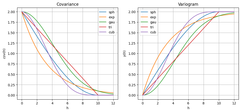
Models: `spherical`, `exponential`, `gaussian`, `triangular`, `cubic`

[5]:

w = 2.0
r = 10.0
cov_model_sph = gn.covModel.CovModel1D(elem=[('spherical',   {'w':w, 'r':10})], name='sph')
cov_model_exp = gn.covModel.CovModel1D(elem=[('exponential', {'w':w, 'r':10})], name='exp')
cov_model_gau = gn.covModel.CovModel1D(elem=[('gaussian',    {'w':w, 'r':10})], name='gau')
cov_model_tri = gn.covModel.CovModel1D(elem=[('triangular',  {'w':w, 'r':10})], name='tri')
cov_model_cub = gn.covModel.CovModel1D(elem=[('cubic',       {'w':w, 'r':10})], name='cub')

cov_model_list = [cov_model_sph, cov_model_exp, cov_model_gau, cov_model_tri, cov_model_cub]

[6]:

# Print sill and range
for cov_model in cov_model_list:
    print(f'Cov. model {cov_model.name}: sill = {cov_model.sill()}, range = {cov_model.r()}')

Cov. model sph: sill = 2.0, range = 10
Cov. model exp: sill = 2.0, range = 10
Cov. model gau: sill = 2.0, range = 10
Cov. model tri: sill = 2.0, range = 10
Cov. model cub: sill = 2.0, range = 10

[7]:

# Plot covariance and variogram
plt.subplots(1,2, figsize=(12,5))

plt.subplot(1,2,1)
# plot covariance
for cov_model in cov_model_list:
    cov_model.plot_model(label=cov_model.name)
plt.legend()
plt.grid(True)
plt.title('Covariance')

plt.subplot(1,2,2)
# plot variogram
for cov_model in cov_model_list:
    cov_model.plot_model(vario=True, label=cov_model.name)
plt.legend()
plt.grid(True)
plt.title('Variogram')
plt.show()

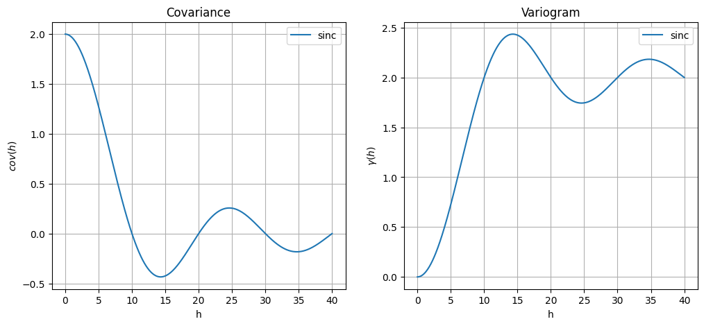
../_images/notebooks_ex_general_multiGaussian_11_0.png

Model: `sinus_cardinal`

[8]:

cov_model_sinc = gn.covModel.CovModel1D(elem=[('sinus_cardinal', {'w':w, 'r':10})], name='sinc')

[9]:

# Print sill and range
cov_model = cov_model_sinc
print(f'Cov. model {cov_model.name}: sill = {cov_model.sill()}, range = {cov_model.r()}')

Cov. model sinc: sill = 2.0, range = 10

[10]:

# Plot covariance and variogram
cov_model = cov_model_sinc

plt.subplots(1,2, figsize=(12,5))

plt.subplot(1,2,1)
# plot covariance
cov_model.plot_model(label=cov_model.name, hmax=4.0*cov_model.r())
plt.legend()
plt.grid(True)
plt.title('Covariance')

plt.subplot(1,2,2)
# plot variogram
cov_model.plot_model(vario=True, label=cov_model.name, hmax=4.0*cov_model.r())
plt.legend()
plt.grid(True)
plt.title('Variogram')
plt.show()

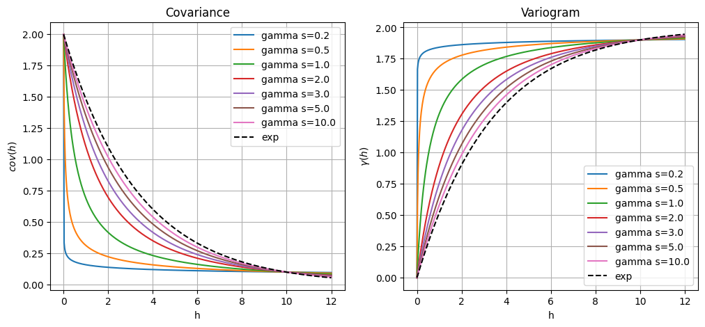
../_images/notebooks_ex_general_multiGaussian_15_0.png

Model: `gamma`

[11]:

w = 2.0
r = 10.0
s_list = [0.2, 0.5, 1.0, 2.0, 3.0, 5.0, 10.0]
cov_model_gamma_list = [
    gn.covModel.CovModel1D(elem=[('gamma', {'w':w, 'r':10, 's':s})], name=f'gamma s={s}')
    for s in s_list]

[12]:

# Print sill and range
for cov_model in cov_model_gamma_list:
    print(f'Cov. model {cov_model.name}: sill = {cov_model.sill()}, range = {cov_model.r()}')

Cov. model gamma s=0.2: sill = 2.0, range = 10
Cov. model gamma s=0.5: sill = 2.0, range = 10
Cov. model gamma s=1.0: sill = 2.0, range = 10
Cov. model gamma s=2.0: sill = 2.0, range = 10
Cov. model gamma s=3.0: sill = 2.0, range = 10
Cov. model gamma s=5.0: sill = 2.0, range = 10
Cov. model gamma s=10.0: sill = 2.0, range = 10

[13]:

# Plot covariance and variogram
plt.subplots(1,2, figsize=(12,5))

plt.subplot(1,2,1)
# plot covariance
for cov_model in cov_model_gamma_list:
    cov_model.plot_model(label=cov_model.name)
cov_model_exp.plot_model(label=cov_model_exp.name, ls='dashed', color='black')
plt.legend()
plt.grid(True)
plt.title('Covariance')

plt.subplot(1,2,2)
# plot variogram
for cov_model in cov_model_gamma_list:
    cov_model.plot_model(vario=True, label=cov_model.name)
cov_model_exp.plot_model(vario=True, label=cov_model_exp.name, ls='dashed', color='black')
plt.legend()
plt.grid(True)
plt.title('Variogram')
plt.show()

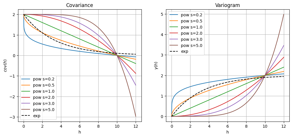
../_images/notebooks_ex_general_multiGaussian_19_0.png

Model: `power`

Warning: this is not a stationary model (does not reach a plateau / sill).

[14]:

w = 2.0
r = 10.0
s_list = [0.2, 0.5, 1.0, 2.0, 3.0, 5.0]
cov_model_pow_list = [
    gn.covModel.CovModel1D(elem=[('power', {'w':w, 'r':10, 's':s})], name=f'pow s={s}')
    for s in s_list]

[15]:

# Print sill and range
for cov_model in cov_model_pow_list:
    print(f'Cov. model {cov_model.name}: sill = {cov_model.sill()}, range = {cov_model.r()}')

Cov. model pow s=0.2: sill = 2.0, range = 10
Cov. model pow s=0.5: sill = 2.0, range = 10
Cov. model pow s=1.0: sill = 2.0, range = 10
Cov. model pow s=2.0: sill = 2.0, range = 10
Cov. model pow s=3.0: sill = 2.0, range = 10
Cov. model pow s=5.0: sill = 2.0, range = 10

[16]:

# Plot covariance and variogram
plt.subplots(1,2, figsize=(12,5))

plt.subplot(1,2,1)
# plot covariance
for cov_model in cov_model_pow_list:
    cov_model.plot_model(label=cov_model.name)
cov_model_exp.plot_model(label=cov_model_exp.name, ls='dashed', color='black')
plt.legend()
plt.grid(True)
plt.title('Covariance')

plt.subplot(1,2,2)
# plot variogram
for cov_model in cov_model_pow_list:
    cov_model.plot_model(vario=True, label=cov_model.name)
cov_model_exp.plot_model(vario=True, label=cov_model_exp.name, ls='dashed', color='black')
plt.legend()
plt.grid(True)
plt.title('Variogram')
plt.show()

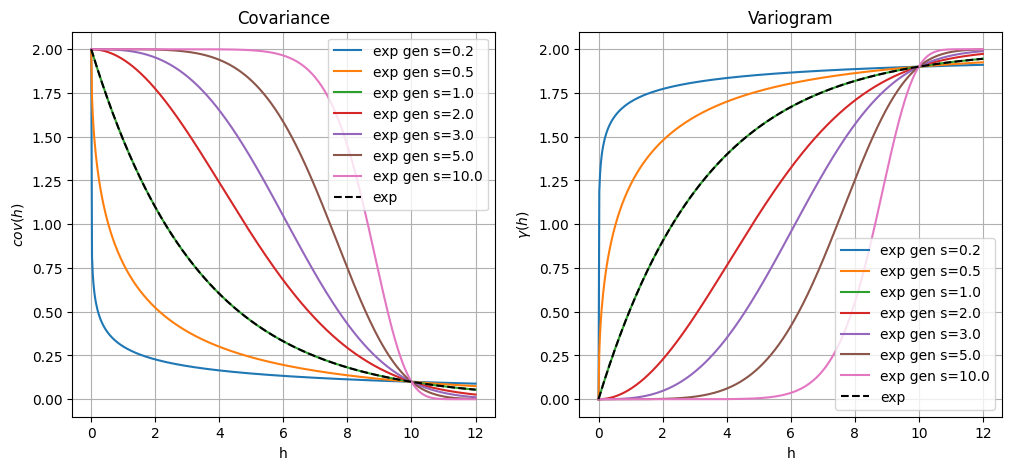
../_images/notebooks_ex_general_multiGaussian_23_0.png

Model: `exponential_generalized`

[17]:

w = 2.0
r = 10.0
s_list = [0.2, 0.5, 1.0, 2.0, 3.0, 5.0, 10.0]
cov_model_exp_gen_list = [
    gn.covModel.CovModel1D(elem=[('exponential_generalized', {'w':w, 'r':10, 's':s})], name=f'exp gen s={s}')
    for s in s_list]

[18]:

# Print sill and range
for cov_model in cov_model_exp_gen_list:
    print(f'Cov. model {cov_model.name}: sill = {cov_model.sill()}, range = {cov_model.r()}')

Cov. model exp gen s=0.2: sill = 2.0, range = 10
Cov. model exp gen s=0.5: sill = 2.0, range = 10
Cov. model exp gen s=1.0: sill = 2.0, range = 10
Cov. model exp gen s=2.0: sill = 2.0, range = 10
Cov. model exp gen s=3.0: sill = 2.0, range = 10
Cov. model exp gen s=5.0: sill = 2.0, range = 10
Cov. model exp gen s=10.0: sill = 2.0, range = 10

[19]:

# Plot covariance and variogram
plt.subplots(1,2, figsize=(12,5))

plt.subplot(1,2,1)
# plot covariance
for cov_model in cov_model_exp_gen_list:
    cov_model.plot_model(label=cov_model.name)
cov_model_exp.plot_model(label=cov_model_exp.name, ls='dashed', color='black')
plt.legend()
plt.grid(True)
plt.title('Covariance')

plt.subplot(1,2,2)
# plot variogram
for cov_model in cov_model_exp_gen_list:
    cov_model.plot_model(vario=True, label=cov_model.name)
cov_model_exp.plot_model(vario=True, label=cov_model_exp.name, ls='dashed', color='black')
plt.legend()
plt.grid(True)
plt.title('Variogram')
plt.show()

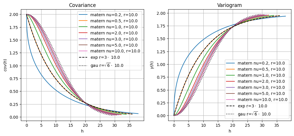
../_images/notebooks_ex_general_multiGaussian_27_0.png

Model: `matern`

Warning: the range is not equal to the parameter ``r``, which is a “scale” parameter.

Covariance matern with parameters w, r, and nu=0.5 is covariance exponential with parameters w, 3r.
Covariance matern with parameters w, r, and nu tends to covariance ‘gaussian’ with parameters w, $\sqrt{6}$ r, when nu tends to infinity.

[20]:

w = 2.0
r = 10.0
nu_list = [0.2, 0.5, 1.0, 2.0, 3.0, 5.0, 10.0]
cov_model_matern_list = [
    gn.covModel.CovModel1D(elem=[('matern', {'w':w, 'r':10, 'nu':nu})], name=f'matern nu={nu}, r={r}')
    for nu in nu_list]

[21]:

# Print sill and range (cov_model.r() gives the range)
for cov_model in cov_model_matern_list:
    print(f'Cov. model {cov_model.name}: sill = {cov_model.sill()}, range = {cov_model.r()}')

Cov. model matern nu=0.2, r=10.0: sill = 2.0, range = 31.63139161186625
Cov. model matern nu=0.5, r=10.0: sill = 2.0, range = 29.957322735539908
Cov. model matern nu=1.0, r=10.0: sill = 2.0, range = 28.27382241179835
Cov. model matern nu=2.0, r=10.0: sill = 2.0, range = 26.841876278504646
Cov. model matern nu=3.0, r=10.0: sill = 2.0, range = 26.19786003151972
Cov. model matern nu=5.0, r=10.0: sill = 2.0, range = 25.590039613951095
Cov. model matern nu=10.0, r=10.0: sill = 2.0, range = 25.065105293108747

[22]:

cov_model_expA = gn.covModel.CovModel1D(elem=[('exponential', {'w':w, 'r':3*r})],
                                        name=r'exp r=$3\cdot$' + f' {r}')
cov_model_gauA = gn.covModel.CovModel1D(elem=[('gaussian', {'w':w, 'r':np.sqrt(6)*r})],
                                        name=r'gau r=$\sqrt{6}\cdot$' + f' {r}')

# Plot covariance and variogram
plt.subplots(1,2, figsize=(12,5))

plt.subplot(1,2,1)
# plot covariance
for cov_model in cov_model_matern_list:
    cov_model.plot_model(label=cov_model.name)
cov_model_expA.plot_model(label=cov_model_expA.name, ls='dashed', color='black')
cov_model_gauA.plot_model(label=cov_model_gauA.name, ls='dotted', color='black')
plt.legend()
plt.grid(True)
plt.title('Covariance')

plt.subplot(1,2,2)
# plot variogram
for cov_model in cov_model_matern_list:
    cov_model.plot_model(vario=True, label=cov_model.name)
cov_model_expA.plot_model(vario=True, label=cov_model_expA.name, ls='dashed', color='black')
cov_model_gauA.plot_model(vario=True, label=cov_model_gauA.name, ls='dotted', color='black')
plt.legend()
plt.grid(True)
plt.title('Variogram')
plt.show()

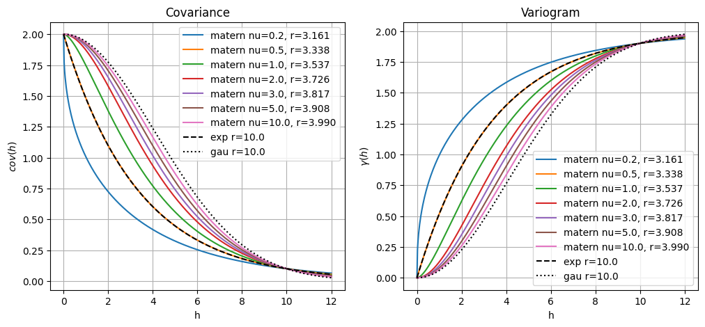
../_images/notebooks_ex_general_multiGaussian_31_0.png

Parameters `r`, `nu` and “effective” range

The function geone.covModel.cov_matern_get_r_param(nu, r_eff) computes the parameter r (scale) such that the 1D-matern covariance model of parameters r and nu has an effective range of r_eff (approximately).

The function geone.covModel.cov_matern_get_effective_range(nu, r) computes the effective range r_eff of a 1D-matern covariance model of parameter r (scale) and nu.

[23]:

r_eff = 10.0
nu_list = [0.2, 0.5, 1.0, 2.0, 3.0, 5.0, 10.0]
r_list = [gn.covModel.cov_matern_get_r_param(nu, r_eff) for nu in nu_list]
for nu, r in zip(nu_list, r_list):
    print(f'nu={nu}, r={r}')

nu=0.2, r=3.1614163937854056
nu=0.5, r=3.3380820069533197
nu=1.0, r=3.5368404930729085
nu=2.0, r=3.725521977764187
nu=3.0, r=3.817105667397543
nu=5.0, r=3.907770425860613
nu=10.0, r=3.9896102103147046

/home/julien/miniconda3/envs/py313/lib/python3.13/site-packages/geone/covModel.py:380: RuntimeWarning: invalid value encountered in scalar power
  u1 = (0.5*u)**nu

[24]:

cov_model_matern_list2 = [
    gn.covModel.CovModel1D(elem=[('matern', {'w':w, 'r':r, 'nu':nu})], name=f'matern nu={nu}, r={r:4.3f}')
    for nu, r in zip(nu_list, r_list)]

[25]:

# Print sill and range (cov_model.r() gives the range)
for cov_model in cov_model_matern_list2:
    print(f'Cov. model {cov_model.name}: sill = {cov_model.sill()}, range = {cov_model.r()}')

Cov. model matern nu=0.2, r=3.161: sill = 2.0, range = 10.00000000000001
Cov. model matern nu=0.5, r=3.338: sill = 2.0, range = 9.999999999999938
Cov. model matern nu=1.0, r=3.537: sill = 2.0, range = 10.000000000000073
Cov. model matern nu=2.0, r=3.726: sill = 2.0, range = 10.000000000000002
Cov. model matern nu=3.0, r=3.817: sill = 2.0, range = 10.000000000000151
Cov. model matern nu=5.0, r=3.908: sill = 2.0, range = 9.999999999999964
Cov. model matern nu=10.0, r=3.990: sill = 2.0, range = 9.99999999999998

[26]:

# Check
a = []
for cov_model in cov_model_matern_list2:
    nu, r = cov_model.elem[0][1]['nu'], cov_model.elem[0][1]['r']
    a.append(cov_model.r() == gn.covModel.cov_matern_get_effective_range(nu, r))

print(np.all(a)) # should be True

True

[27]:

cov_model_expB = gn.covModel.CovModel1D(elem=[('exponential', {'w':w, 'r':r_eff})], name=f'exp r={r_eff}')
cov_model_gauB = gn.covModel.CovModel1D(elem=[('gaussian', {'w':w, 'r':r_eff})], name=f'gau r={r_eff}')

# Plot covariance and variogram
plt.subplots(1,2, figsize=(12,5))

plt.subplot(1,2,1)
# plot covariance
for cov_model in cov_model_matern_list2:
    cov_model.plot_model(label=cov_model.name)
cov_model_expB.plot_model(label=cov_model_expB.name, ls='dashed', color='black')
cov_model_gauB.plot_model(label=cov_model_gauB.name, ls='dotted', color='black')
plt.legend()
plt.grid(True)
plt.title('Covariance')

plt.subplot(1,2,2)
# plot variogram
for cov_model in cov_model_matern_list2:
    cov_model.plot_model(vario=True, label=cov_model.name)
cov_model_expB.plot_model(vario=True, label=cov_model_expB.name, ls='dashed', color='black')
cov_model_gauB.plot_model(vario=True, label=cov_model_gauB.name, ls='dotted', color='black')
plt.legend()
plt.grid(True)
plt.title('Variogram')
plt.show()

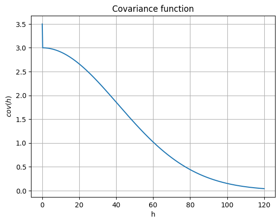
../_images/notebooks_ex_general_multiGaussian_37_0.png

Defining a covariance model in 1D: class `geone.covModel.covModel1D`

A covariance model is defined by its elementary contributions given as a list of 2-tuples, whose the first component is the type given by a string (nugget, spherical, exponential, gaussian, …) and the second component is a dictionary used to pass the required parameters (the weight (w), the range (r), …).

Example

[28]:

cov_model = gn.covModel.CovModel1D(elem=[
    ('gaussian', {'w':3.0, 'r':100}), # elementary contribution
    ('nugget', {'w':.5})              # elementary contribution
    ], name='model-1D example')

print(cov_model)

*** CovModel1D object ***
name = 'model-1D example'
number of elementary contribution(s): 2
elementary contribution 0
    type: gaussian
    parameters:
        w = 3.0
        r = 100
elementary contribution 1
    type: nugget
    parameters:
        w = 0.5
*****

Plot the covariance / variogram function of the model

Note: plotting is not available for non-stationary covariance model.

[29]:

plt.figure()
cov_model.plot_model()
plt.title('Covariance function')
plt.show()

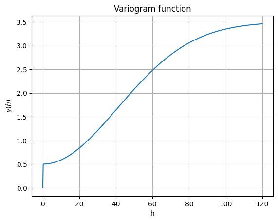
../_images/notebooks_ex_general_multiGaussian_42_0.png

[30]:

plt.figure()
cov_model.plot_model(vario=True)
plt.title('Variogram function')
plt.show()

../_images/notebooks_ex_general_multiGaussian_43_0.png

[31]:

plt.figure()
cov_model.plot_model(label='covar.')
cov_model.plot_model(vario=True, label='vario.')
plt.legend()
plt.title('Variogram function')
plt.show()

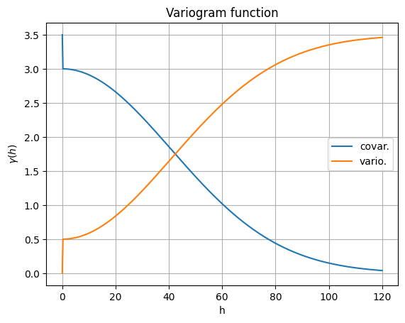
../_images/notebooks_ex_general_multiGaussian_44_0.png

Get the sill and range

[32]:

w = cov_model.sill()
r = cov_model.r()
print(f'Sill = {w}')
print(f'Range = {r}')

Sill = 3.5
Range = 100

Defining a covariance model in 2D: class `geone.covModel.covModel2D`

A covariance model is defined by its elementary contributions given as a list of 2-tuples, whose the first component is the type given by a string (nugget, spherical, exponential, gaussian, …) and the second component is a dictionary used to pass the required parameters (the weight (w), the range (r), …).

An azimuth angle, alpha, can be specified in degrees: the coordinates system Ox’y’ supporting the axes of the model (ranges) is obtained from the original coordinates system Oxy by applying a rotation of -alpha (i.e. clockwise for positive angle).

[33]:

cov_model = gn.covModel.CovModel2D(elem=[
    ('spherical', {'w':5., 'r':[150, 40]}), # elementary contribution
    ('nugget', {'w':.5})                    # elementary contribution
    ], alpha=-30, name='model-2D example')

print(cov_model)

*** CovModel2D object ***
name = 'model-2D example'
number of elementary contribution(s): 2
elementary contribution 0
    type: spherical
    parameters:
        w = 5.0
        r = [150, 40]
elementary contribution 1
    type: nugget
    parameters:
        w = 0.5
angle: alpha = -30 deg.
    i.e.: the system Ox'y', supporting the axes of the model (ranges),
    is obtained from the system Oxy by applying a rotation of angle -alpha.
*****

Plot the covariance / variogram function of the model

Plot the covariance function by using the method plot_model of the class. The following keyword arguments controls what is plotted:

plot_map: True (default) or False indicating if the 2D-map is plotted
plot_curves: True (default) or False indicating if curves of the function along axes x’ and y’ are plotted

If both are plot_map and plot_curves are set to True a new 1x2 figure is created (the size of the figure can be set with the keyword arguments figsize (tuple of 2 ints) and the keyword argument show_suptitle (True (default) or False) indicates if characteristics of the model is displayed as sup-title).

If only one of plot_map and plot_curves is set to True, the plot is done in the current figure axis.

Note: plotting is not available for non-stationary covariance model.

[34]:

cov_model.plot_model(figsize=(15,5))
plt.suptitle('')
plt.show()

../_images/notebooks_ex_general_multiGaussian_51_0.png

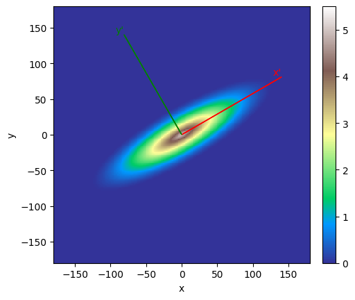
[35]:

plt.figure()
cov_model.plot_model(plot_map=True, plot_curves=False)
plt.show()

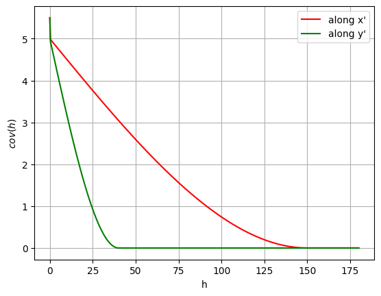
../_images/notebooks_ex_general_multiGaussian_52_0.png

[36]:

plt.figure()
cov_model.plot_model(plot_map=False, plot_curves=True)
plt.show()

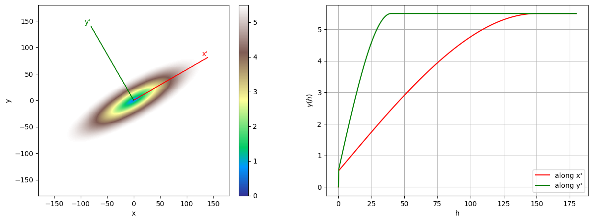
../_images/notebooks_ex_general_multiGaussian_53_0.png

Plot the variogram function. Same as above, but passing the keyword argument vario=True to the method plot_model.

[37]:

cov_model.plot_model(vario=True, figsize=(15,5))
plt.suptitle('')
plt.show()

../_images/notebooks_ex_general_multiGaussian_55_0.png

The main axes x’ and y’ can be plotted using the method plot_mrot.

[38]:

plt.figure()
cov_model.plot_mrot()
plt.show()

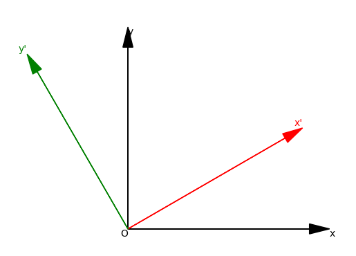
../_images/notebooks_ex_general_multiGaussian_57_0.png

Note that the colors used for the main axes (x’ and y’) can be changed in the figures above by passing the keyword arguments color0 (axis x’) and color1 (axis y’).

Get the sill and ranges

Get the sill and the range along each axis in the coordinates system supporting the axes of the model.

[39]:

w = cov_model.sill() # scalar
r = cov_model.r12()  # vector (1d-array) of length 2: ranges along x', y'
print(f"Sill = {w}")
print(f"Range along x' = {r[0]}, along y' = {r[1]}")

Sill = 5.5
Range along x' = 150.0, along y' = 40.0

Get the maximal range along each axis of the original system Oxy.

[40]:

rxy = cov_model.rxy()  # vector (1d-array) of length 2: "max ranges" along x, y
print(f"Max. range along x = {rxy[0]}, along y = {rxy[1]}")

Max. range along x = 129.9038105676658, along y = 74.99999999999999

Defining a covariance model in 3D: class `geone.covModel.covModel3D`

A covariance model is defined by its elementary contributions given as a list of 2-tuples, whose the first component is the type given by a string (nugget, spherical, exponential, gaussian, …) and the second component is a dictionary used to pass the required parameters (the weight (w), the range (r), …).

Azimuth (alpha), dip (beta) and plunge (gamma) angles can be specified in degrees: the coordinates system Ox’’’y’’’’z’’’, supporting the axes of the model (ranges), is obtained from the original coordinates system Oxyz as follows:

Oxyz -> rotation of angle -alpha around Oz -> Ox’y’z’
Ox’y’z’ -> rotation of angle -beta around Ox’ -> Ox’’y’’z’’
Ox’’y’’z’’ -> rotation of angle -gamma around Oy’’ -> Ox’’’y’’’z’’’

[41]:

cov_model = gn.covModel.CovModel3D(elem=[
    ('gaussian', {'w':8.5, 'r':[40, 20, 10]}), # elementary contribution
    ('nugget', {'w':0.5})                      # elementary contribution
    ], alpha=-30, beta=-40, gamma=20, name='model-3D example')

[42]:

cov_model

[42]:

*** CovModel3D object ***
name = 'model-3D example'
number of elementary contribution(s): 2
elementary contribution 0
    type: gaussian
    parameters:
        w = 8.5
        r = [40, 20, 10]
elementary contribution 1
    type: nugget
    parameters:
        w = 0.5
angles: alpha = -30, beta = -40, gamma = 20 (in degrees)
    i.e.: the system Ox'''y''''z''', supporting the axes of the model (ranges),
    is obtained from the system Oxyz as follows:
        Oxyz      -- rotation of angle -alpha around Oz  --> Ox'y'z'
        Ox'y'z'   -- rotation of angle -beta  around Ox' --> Ox''y''z''
        Ox''y''z''-- rotation of angle -gamma around Oy''--> Ox'''y'''z'''
*****

Plot the covariance / variogram function of the model

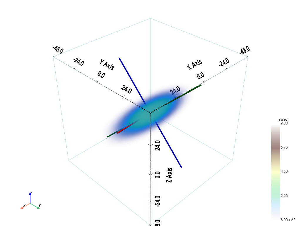
Plot the covariance function by using the method plot_model3d_volume of the class for a 3D volume representation (based on pyvista module). The main axes are shown in red (x’’’), green (y’’’) and blue (z’’’’), or in custom colors passing the keyword arguments color0 (x’’’), color1 (y’’’), and color2 (z’’’).

Note: plotting is not available for non-stationary covariance model.

[43]:

cov_model.plot_model3d_volume()

../_images/notebooks_ex_general_multiGaussian_69_0.png

For a view in an intaractive figure (pop-up window):

[44]:

%%script false --no-raise-error # skip this cell! (comment this line to run the cell)

pp = pv.Plotter(notebook=False) # open a plotter and specifying 'notebook=False'
cov_model.plot_model3d_volume(plotter=pp)
pp.show() # after closing the pop-up window, the position of the camera is retrieved in output.

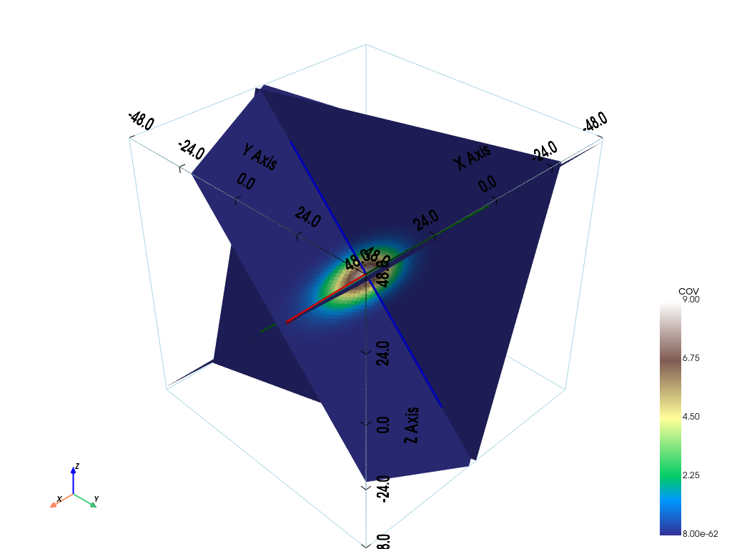
The method plot_model3d_slice of the class gives a 3D representations with slices orthogonal to the main axes and going through the origin (by default).

[45]:

cov_model.plot_model3d_slice()

../_images/notebooks_ex_general_multiGaussian_73_0.png

[46]:

%%script false --no-raise-error # skip this cell! (comment this line to run the cell)

# Interactive figure
pp = pv.Plotter(notebook=False) # open a plotter and specifying 'notebook=False'
cov_model.plot_model3d_slice(plotter=pp)
pp.show() # after closing the pop-up window, the position of the camera is retrieved in output.

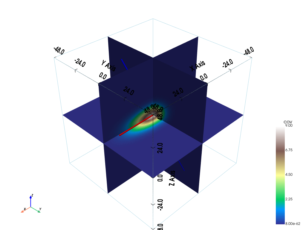
For plotting slices orthogonal to each axis of the system Oxyz:

[47]:

cov_model.plot_model3d_slice(slice_normal_x=0, slice_normal_y=0, slice_normal_z=0, slice_normal_custom=None)

../_images/notebooks_ex_general_multiGaussian_76_0.png

[48]:

%%script false --no-raise-error # skip this cell! (comment this line to run the cell)

# Interactive figure
pp = pv.Plotter(notebook=False) # open a plotter and specifying 'notebook=False'
cov_model.plot_model3d_slice(plotter=pp,
                             slice_normal_x=0, slice_normal_y=0, slice_normal_z=0, slice_normal_custom=None)
pp.show() # after closing the pop-up window, the position of the camera is retrieved in output.

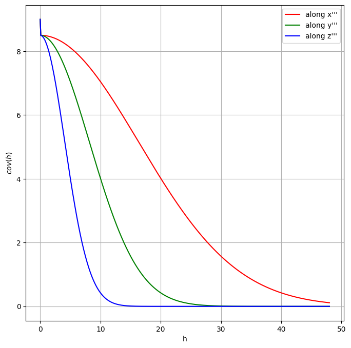
Plot the covariance function by using the method plot_model_curves of the class for plotting the function along each main axis (x’’’, y’’’, and z’’’). Again, the default colors can be changed by passing the keyword arguments color0, color1, and color2.

[49]:

plt.figure(figsize=(8,8))
cov_model.plot_model_curves()
plt.show()

../_images/notebooks_ex_general_multiGaussian_79_0.png

Plotting the variogram function: as above, but passing the keyword argument vario=True to the method plot_model3d_volume or plot_model3d_sclice or plot_model_curves.

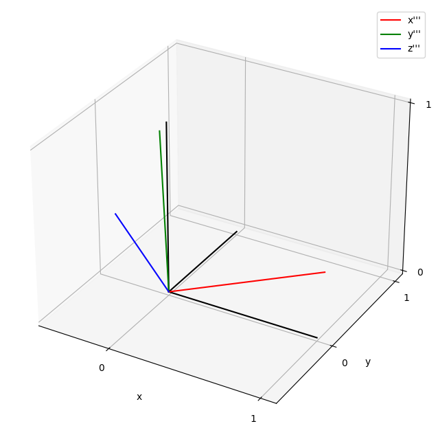
The main axes (x’’’, y’’’ and z’’’) can be plotted using the method plot_mrot. Again, the default colors can be changed by passing the keyword arguments color0, color1, and color2.

[50]:

cov_model.plot_mrot(figsize=(8,8))

../_images/notebooks_ex_general_multiGaussian_82_0.png

Get the sill and ranges

Get the sill and the range along each axis in the coordinates system supporting the axes of the model.

[51]:

w = cov_model.sill() # scalar
r = cov_model.r123() # vector (1d-array) of length 3 ranges along x'''', y''', z'''
print("Sill = {}".format(w))
print("Range along x''' = {}, along y''' = {}, along z''' = {}".format(r[0], r[1], r[2]))

Sill = 9.0
Range along x''' = 40.0, along y''' = 20.0, along z''' = 10.0

Get the maximal range along each axis of the original system Oxyz.

[52]:

rxyz = cov_model.rxyz()  # vector (1d-array) of length 2: "max ranges" along x, y, z
print("Max. range along x = {}, along y = {}, along z = {}".format(rxyz[0], rxyz[1], rxyz[2]))

Max. range along x = 36.948833461834035, along y = 13.268278963378767, along z = 12.855752193730785

GEONE - multiGaussian estimation and simulation

Functions for kriging and SGS in a grid

Kriging

SGS

Output

One wrapper: function geone.multiGaussian.multiGaussianRun

Covariance model

Available elementary covariance models (1D)

Import what is required

Remark

Models: spherical, exponential, gaussian, triangular, cubic

Model: sinus_cardinal

Model: gamma

Model: power

Model: exponential_generalized

Model: matern

Parameters r, nu and “effective” range

Defining a covariance model in 1D: class geone.covModel.covModel1D

Example

Plot the covariance / variogram function of the model

Get the sill and range

Defining a covariance model in 2D: class geone.covModel.covModel2D

Plot the covariance / variogram function of the model

Get the sill and ranges

Defining a covariance model in 3D: class geone.covModel.covModel3D

Plot the covariance / variogram function of the model

Get the sill and ranges

One wrapper: function `geone.multiGaussian.multiGaussianRun`

Models: `spherical`, `exponential`, `gaussian`, `triangular`, `cubic`

Model: `sinus_cardinal`

Model: `gamma`

Model: `power`

Model: `exponential_generalized`

Model: `matern`

Parameters `r`, `nu` and “effective” range

Defining a covariance model in 1D: class `geone.covModel.covModel1D`

Defining a covariance model in 2D: class `geone.covModel.covModel2D`

Defining a covariance model in 3D: class `geone.covModel.covModel3D`