GEONE - Tools to deal with 2D RGB images
Functions to read, write and show images 2D RGB images:
read from file in format png, ppm, (jpeg),
link with geone image (
geone.img.Imgclass).
Use package Pillow (PIL) for advanced image manipulation and various file formats.
Import what is required
[1]:
import numpy as np
import matplotlib.pyplot as plt
import os

# import package 'geone'
import geone as gn
[2]:
# Show version of python and version of geone
import sys
print(sys.version_info)
print('geone version: ' + gn.__version__)
sys.version_info(major=3, minor=13, micro=7, releaselevel='final', serial=0)
geone version: 1.3.1
Read / Write 2D RGB image files
The function geone.img.readImage2Drgb allows to read (load) 2D images with RGB (or RGBA) channels from file in various format (png, ppm(, jpeg)) (based on matplotlib.pyplot.imread) and to fill an instance of geone.img.Img class.
The function geone.img.writeImage2Drgb allows to write (save) an image (based on matplotlib.pyplot.imsave) from a geone.img.Img class instance in a file, in format png, ppm(, jpeg). The input image (geone.img.Img class) should be in 2D with one variable, 3 variables (channels RGB) or 4 variables (channels RGBA). If the input image has only one variable, it is transformed in a RGB(A) color code via a list of color or a colormap.
See examples below for more details.
Notes:
geone.img.readImage2Drgb(matplotlib.pyplot.imread) allows more file format thangeone.img.writeImage2Drgb(matplotlib.pyplot.imsave), e.g. ‘tif’,format ‘jpeg’ renders blurred images, so they should avoid at least for categorical images.
Dealing with “missing value”
The function geone.img.readImage2Drgb allows to specify a color that is considered as a “missing value” (coded by nan) in the output geone image.
The function geone.img.writeImage2Drgb allows to specify the color to be used for “missing_value” (nan) in the input geone image.
See examples below for more details.
[3]:
# Set output directory for generated files
out_dir = 'out'

if not os.path.isdir(out_dir):
    os.mkdir(out_dir)
I. Example with “continuous” image
Reading / loading image
The function geone.img.readImage2Drgb returns an image (geone.img.Img class) with:
3 or 4 variables (keyword argument
keep_channels=True(default)), the variables (with value in the interval![[0, 1]](../_images/math/8027137b3073a7f5ca4e45ba2d030dcff154eca4.png) ) being the RGB or RGBA channels,
) being the RGB or RGBA channels,1 variable (keyword argument
keep_channels=False), the variable (with value in the interval) being a linear combination of the RGB channels using the weight given by the keyword argument rgb_weight.
[4]:
# Directory containing the input files
data_dir = 'data'

# Filename of the initial image, without extension
fbase = 'imCont'

# Extension
ext = 'png'
I. 1 Continuous image - keeping RGB(A) channels
Read file with matplotlib.pyplot.imread and show it with matplotlib.pyplot.imshow
[5]:
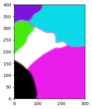
# Read the image from initial file using matplotlib.pyplot.imread and show it
im = plt.imread(os.path.join(data_dir, f'{fbase}.{ext}'))
plt.figure(figsize=(4,4))
plt.imshow(im)
plt.axis('off')
plt.show()

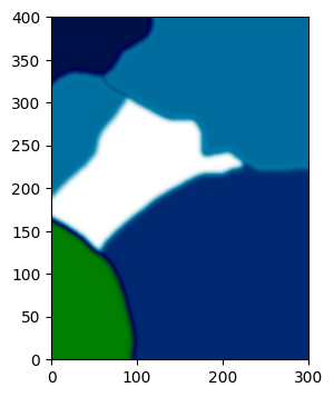
Read file using dedicated function of geone (geone.img.readImage2Drgb)
[6]:
# Read the image from initial file, keeping RGB(A) channels
im_cont = gn.img.readImage2Drgb(os.path.join(data_dir, f'{fbase}.{ext}'))

# Show info
print('Geone image (gn.img.Img):\n', im_cont)
Geone image (gn.img.Img):
 *** Img object ***
name = ''
(nx, ny, nz) = (300, 400, 1) # number of cells along each axis
(sx, sy, sz) = (1.0, 1.0, 1.0) # cell size (spacing) along each axis
(ox, oy, oz) = (0.0, 0.0, 0.0) # origin (coordinates of bottom-lower-left corner)
nv = 3  # number of variable(s)
varname = [np.str_('red'), np.str_('green'), np.str_('blue')]
val: (3, 1, 400, 300)-array
*****
[7]:
# Plot the image with gn.imgplot.drawImage2Drgb (recombining the RGB(A) channels)
plt.figure(figsize=(4,4))
gn.imgplot.drawImage2Drgb(im_cont)
plt.show()
[8]:
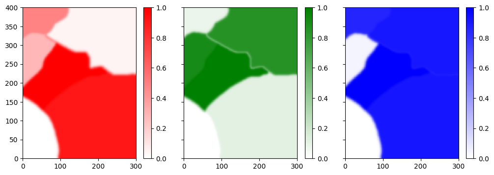
# Plot the three variables (RGB channels) of the image with gn.imgplot.drawImage2D
plt.subplots(1,3, sharey=True, figsize=(12,4))
plt.subplot(1,3,1)
gn.imgplot.drawImage2D(im_cont, iv=0, cmap=gn.customcolors.custom_cmap(['white', 'red']))
plt.subplot(1,3,2)
gn.imgplot.drawImage2D(im_cont, iv=1, cmap=gn.customcolors.custom_cmap(['white', 'green']))
plt.subplot(1,3,3)
gn.imgplot.drawImage2D(im_cont, iv=2, cmap=gn.customcolors.custom_cmap(['white', 'blue']))
plt.show()
Writing / saving image
[9]:
# output file
out_file = f'{fbase}_new.{ext}'
f = os.path.join(out_dir, out_file)
gn.img.writeImage2Drgb(f, im_cont)

# Read the image from the written file
im_cont_new = gn.img.readImage2Drgb(f)
if im_cont.nv == 3:
    im_cont_new.resize(iv0=0, iv1=3) # keep only the first three channels (remove alpha channel)
print('Same geone images (im_cont and im_cont_new) ?', gn.img.isImageEqual(im_cont, im_cont_new))
Same geone images (im_cont and im_cont_new) ? True
[10]:
# Note: if the image read with matplotlib.pyplot.imread is saved with matplotlib.pyplot.imsave,
# we get the same file as the file written just above

# output file
out_file = f'{fbase}_copy.{ext}'
f = os.path.join(out_dir, out_file)
plt.imsave(f, im)
Dealing with missing value
[11]:
nancol = im_cont.val[:,0,0,0] # color code of first pixel (in bottom left corner), in initial image

# Read the image from the initial file, specifying a color to be interpreted as missing value
im_cont_x = gn.img.readImage2Drgb(os.path.join(data_dir, f'{fbase}.{ext}'), nancol=nancol)

print('Number of pixel with missing value: ', np.any(np.isnan(im_cont_x.val), axis=0).sum())
Number of pixel with missing value: 9606
[12]:
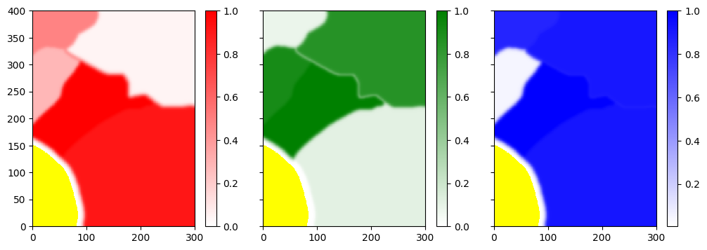
# Plot the three variables (RGB channels) of the image with gn.imgplot.drawImage2D
# (with missing value in yellow)
plt.subplots(1,3, sharey=True, figsize=(12,4))
plt.subplot(1,3,1)
gn.imgplot.drawImage2D(im_cont_x, iv=0, cmap=gn.customcolors.custom_cmap(['white', 'red'], cbad='yellow'))
plt.subplot(1,3,2)
gn.imgplot.drawImage2D(im_cont_x, iv=1, cmap=gn.customcolors.custom_cmap(['white', 'green'], cbad='yellow'))
plt.subplot(1,3,3)
gn.imgplot.drawImage2D(im_cont_x, iv=2, cmap=gn.customcolors.custom_cmap(['white', 'blue'], cbad='yellow'))
plt.show()
[13]:
# Write image accounting for missing value
out_file = f'{fbase}_x_new.{ext}' # output file
f = os.path.join(out_dir, out_file)
gn.img.writeImage2Drgb(f, im_cont_x, nancol='yellow')

# Read the image from the written file
im_cont_x_new = gn.img.readImage2Drgb(f, nancol='yellow')
if im_cont_x.nv == 3:
    im_cont_x_new.resize(iv0=0, iv1=3) # keep only the first three channels (remove alpha channel)
print('Same geone images (im_cont_x and im_cont_x_new) ?', gn.img.isImageEqual(im_cont_x, im_cont_x_new))
Same geone images (im_cont_x and im_cont_x_new) ? True
I. 2 Continuous image - combining RGB channels
[14]:
# Read the image from the initial file, combining RGB channels: one output variable consisting
# of a linear combination of the RGB code of the color in the original file; weight of RGB channels
# are set with keyword argument 'rgb_weight'
im_cont_onevar = gn.img.readImage2Drgb(os.path.join(data_dir, f'{fbase}.{ext}'), keep_channels=False)

# Show info
print('Geone image (gn.img.Img):\n', im_cont_onevar)
Geone image (gn.img.Img):
 *** Img object ***
name = ''
(nx, ny, nz) = (300, 400, 1) # number of cells along each axis
(sx, sy, sz) = (1.0, 1.0, 1.0) # cell size (spacing) along each axis
(ox, oy, oz) = (0.0, 0.0, 0.0) # origin (coordinates of bottom-lower-left corner)
nv = 1  # number of variable(s)
varname = [np.str_('val')]
val: (1, 1, 400, 300)-array
*****
[15]:
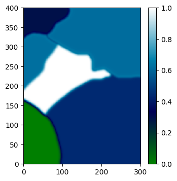
# Draw the image using a color map
plt.figure(figsize=(4,4))
gn.imgplot.drawImage2D(im_cont_onevar, cmap='ocean')
plt.show()
Writing / saving image
The RGB colors in the written file are set via a color map.
[16]:
# output file
out_file = f'{fbase}_onevar_new.{ext}'
f = os.path.join(out_dir, out_file)
gn.img.writeImage2Drgb(f, im_cont_onevar, cmap='ocean')

# Read the image from the written file (keeping RGB(A) channels) and plot it (recombining the RGB(A) channels)
im_cont_onevar_new = gn.img.readImage2Drgb(f) # keeping channels
plt.figure(figsize=(4,4))
gn.imgplot.drawImage2Drgb(im_cont_onevar_new)
plt.show()
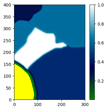
Dealing with missing value
[17]:
nancol = im_cont.val[:,0,0,0] # color code of first pixel (in bottom left corner), in initial image

# Read the image from the initial file, specifying a color to be interpreted as missing value
im_cont_onevar_x = gn.img.readImage2Drgb(os.path.join(data_dir, f'{fbase}.{ext}'),
                                         nancol=nancol, keep_channels=False)

print('Number of pixel with missing value: ', np.any(np.isnan(im_cont_onevar_x.val), axis=0).sum())
Number of pixel with missing value: 9606
[18]:
# Draw the image using a color map
# Define a color map from "ocean color map" and specifying a color for missing value (nan)
cmap = gn.customcolors.custom_cmap([plt.get_cmap('ocean')(x) for x in np.linspace(0,1,256)], ncol=256,
                                   cbad='yellow')

plt.figure(figsize=(4,4))
gn.imgplot.drawImage2D(im_cont_onevar_x, cmap=cmap)
plt.show()
[19]:
# Write image accounting for missing value
out_file = f'{fbase}_onevar_x_new.{ext}' # output file
f = os.path.join(out_dir, out_file)
gn.img.writeImage2Drgb(f, im_cont_onevar_x, cmap=cmap, nancol='yellow')

# Read the image from the written file (keeping RGB(A) channels) and plot it (recombining the RGB(A) channels)
im_cont_onevar_x_new = gn.img.readImage2Drgb(f) # keeping channels
plt.figure(figsize=(4,4))
gn.imgplot.drawImage2Drgb(im_cont_onevar_x_new)
plt.show()

II. Example with “categorical” image
Reading / loading image
If the image is considered as categorical (keyword argument categ=True), the function geone.img.readImage2Drgb returns an image (geone.img.Img class) with one variable taking values being indices (starting from  ), where an index refers to the color of the pixel in a list of colors also retrieved in output. Each color in the list consists in a RGB or RGBA code (sequence of length 3 or 4 of values in ) (keyword argument
 keep_channels=True (default)) or a
float in ![[0,1]](../_images/math/a7b17d1c3442224393b5a845ae344dbe542593d7.png) resulting of a linear combination of the RGB code of the color (keyword argument
resulting of a linear combination of the RGB code of the color (keyword argument keep_channels=False) using the weight given by the keyword argument rgb_weight. The output image im can be drawn (plotted) directly according to the output list of colors col by using:
geone.imgplot.drawImage2D(im, categ=True, categCol=col)if keyword argumentkeep_channelswasTrue;geone.imgplot.drawImage2D(im, categ=True, categCol=[cmap(c) for c in col]), wherecmapis a color map function defined on the interval [0, 1], if keyword argumentkeep_channelswasFalse.
[20]:
# Filename of the initial image, without extension
fbase = 'imCat'

# Extension
ext = 'png'
II. 1 Categorical image - keeping RGB(A) channels
Read file with matplotlib.pyplot.imread and show it with matplotlib.pyplot.imshow
[21]:
# Read the image from the initial file using matplotlib.pyplot.imread and show it
im = plt.imread(os.path.join(data_dir, f'{fbase}.{ext}'))
plt.figure(figsize=(4,4))
plt.imshow(im)
plt.axis('off')
plt.show()

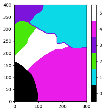
Read file using dedicated function of geone (geone.img.readImage2Drgb)
[22]:
# Read the image from the initial file and retrieve the geone image and the list of colors (RGBA code)
im_cat, col = gn.img.readImage2Drgb(os.path.join(data_dir, f'{fbase}.{ext}'), categ=True)

# Show info
print('Geone image (gn.img.Img):\n', im_cat)
print('Values of the variable (index of colors):', np.unique(im_cat.val))
print('List of colors (RGB(A) code):')
col
Geone image (gn.img.Img):
 *** Img object ***
name = ''
(nx, ny, nz) = (300, 400, 1) # number of cells along each axis
(sx, sy, sz) = (1.0, 1.0, 1.0) # cell size (spacing) along each axis
(ox, oy, oz) = (0.0, 0.0, 0.0) # origin (coordinates of bottom-lower-left corner)
nv = 1  # number of variable(s)
varname = [np.str_('code')]
val: (1, 1, 400, 300)-array
*****
Values of the variable (index of colors): [0. 1. 2. 3. 4. 5.]
List of colors (RGB(A) code):
[22]:
[array([0., 0., 0.], dtype=float32),
 array([0.04313726, 0.8509804 , 0.9098039 ], dtype=float32),
 array([0.28235295, 0.9098039 , 0.04313726], dtype=float32),
 array([0.4862745 , 0.07843138, 0.85882354], dtype=float32),
 array([0.9137255 , 0.10980392, 0.91764706], dtype=float32),
 array([1., 1., 1.], dtype=float32)]
[23]:
# Plot the image with gn.imgplot.drawImage2D
plt.figure(figsize=(4,4))
gn.imgplot.drawImage2D(im_cat, categ=True, categCol=col)
plt.show()
Writing / saving image
[24]:
# output file
out_file = f'{fbase}_new.{ext}'
f = os.path.join(out_dir, out_file)
gn.img.writeImage2Drgb(f, im_cat, col=col)

# Read the image from the written file
im_cat_new, col_new = gn.img.readImage2Drgb(f, categ=True)
print('Same geone images (im_cat and im_cat_new) ?', gn.img.isImageEqual(im_cat, im_cat_new))
print('Same colors (col and col_new) ?', np.all([c[0:3] == cb[0:3] for c, cb in zip(col, col_new)]))
Same geone images (im_cat and im_cat_new) ? True
Same colors (col and col_new) ? True
[25]:
# Note: if the image read with matplotlib.pyplot.imread is saved with matplotlib.pyplot.imsave,
# we get the same file as the file written just above

# output file
out_file = f'{fbase}_copy.{ext}'
f = os.path.join(out_dir, out_file)
plt.imsave(f, im)
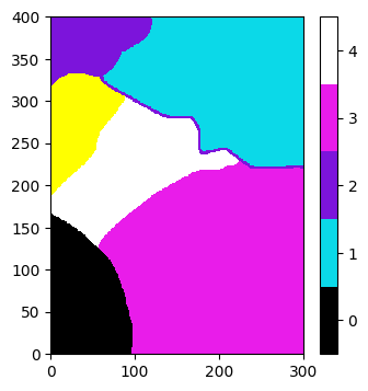
Dealing with missing value
[26]:
nancol = col[2] # color code of the category "2" in initial image

# Read the image from the initial file, specifying a color to be interpreted as missing value
im_cat_x, col_x = gn.img.readImage2Drgb(os.path.join(data_dir, f'{fbase}.{ext}'), categ=True, nancol=nancol)

# Show info
print('Geone image (gn.img.Img):\n', im_cat_x)
print('Values of the variable (index of colors):', np.unique(im_cat_x.val))
print('List of colors (RGB(A) code):')
col_x
Geone image (gn.img.Img):
 *** Img object ***
name = ''
(nx, ny, nz) = (300, 400, 1) # number of cells along each axis
(sx, sy, sz) = (1.0, 1.0, 1.0) # cell size (spacing) along each axis
(ox, oy, oz) = (0.0, 0.0, 0.0) # origin (coordinates of bottom-lower-left corner)
nv = 1  # number of variable(s)
varname = [np.str_('code')]
val: (1, 1, 400, 300)-array
*****
Values of the variable (index of colors): [ 0.  1.  2.  3.  4. nan]
List of colors (RGB(A) code):
[26]:
[array([0., 0., 0.]),
 array([0.04313726, 0.8509804 , 0.90980393]),
 array([0.48627451, 0.07843138, 0.85882354]),
 array([0.9137255 , 0.10980392, 0.91764706]),
 array([1., 1., 1.])]
[27]:
# Plot the image with gn.imgplot.drawImage2D (with missing value in yellow)
plt.figure(figsize=(4,4))
gn.imgplot.drawImage2D(im_cat_x, categ=True, categCol=col_x, categColbad='yellow')
plt.show()
[28]:
# Write image accounting for missing value
out_file = f'{fbase}_x_new.{ext}' # output file
f = os.path.join(out_dir, out_file)
gn.img.writeImage2Drgb(f, im_cat_x, col=col_x, nancol='yellow')

# Read the image from the written file
im_cat_x_new, col_x_new = gn.img.readImage2Drgb(f, categ=True, nancol='yellow')
print('Same geone images (im_cat_x_new and im_cat_x_new) ?', gn.img.isImageEqual(im_cat_x, im_cat_x_new))
print('Same colors (col_x and col_x_new) ?', np.all([c[0:3] == cb[0:3] for c, cb in zip(col_x, col_x_new)]))
Same geone images (im_cat_x_new and im_cat_x_new) ? True
Same colors (col_x and col_x_new) ? True
II. 2 Categorical image - combining RGB channels
[29]:
# Read the image from the initial file and retrieve the geone image and the list of colors.
# Each color is a number in [0,1], resulting of a linear combination of the RGB code of the color
# in the original file; weight of RGB channels are set with keyword argument 'rgb_weight'
im_cat_b, col_b = gn.img.readImage2Drgb(os.path.join(data_dir, f'{fbase}.{ext}'),
                                        categ=True, keep_channels=False)

# Show info
print('Same geone images (im_cat and im_cat_b) ?', gn.img.isImageEqual(im_cat, im_cat_b))
print('List of colors (rate in [0,1]):', col_b)
Same geone images (im_cat and im_cat_b) ? True
List of colors (rate in [0,1]): [0.         0.61614118 0.62339609 0.28934118 0.44227059 1.        ]
[30]:
# Get RGB(A) colors via a color map
cmap = plt.get_cmap('gray')
col_b_rgb = [cmap(c) for c in col_b]
col_b_rgb
[30]:
[(np.float64(0.0), np.float64(0.0), np.float64(0.0), np.float64(1.0)),
 (np.float64(0.615686274509804),
  np.float64(0.615686274509804),
  np.float64(0.615686274509804),
  np.float64(1.0)),
 (np.float64(0.6235294117647059),
  np.float64(0.6235294117647059),
  np.float64(0.6235294117647059),
  np.float64(1.0)),
 (np.float64(0.2901960784313725),
  np.float64(0.2901960784313725),
  np.float64(0.2901960784313725),
  np.float64(1.0)),
 (np.float64(0.44313725490196076),
  np.float64(0.44313725490196076),
  np.float64(0.44313725490196076),
  np.float64(1.0)),
 (np.float64(1.0), np.float64(1.0), np.float64(1.0), np.float64(1.0))]
[31]:
# Plot the image with gn.imgplot.drawImage2D
plt.figure(figsize=(4,4))
gn.imgplot.drawImage2D(im_cat_b, categ=True, categCol=col_b_rgb)
plt.show()
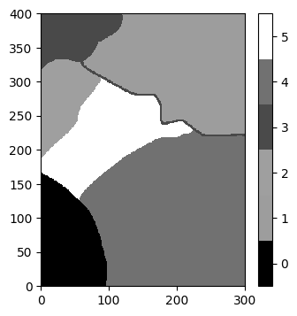
Note that due to the linear combination of RGB channels, the output colors can be very close.
Writing / saving image
The RGB colors in the written file can be first defined via a color map.
[32]:
# output file
out_file = f'{fbase}_b_new.{ext}'
f = os.path.join(out_dir, out_file)
gn.img.writeImage2Drgb(f, im_cat_b, col=col_b_rgb) # use RGB(A) colors defined in col_b_rgb

# Read the image from the written file (keeping RGB(A) channels) and plot it (recombining the RGB(A) channels)
im_cat_b_new, col_b_new = gn.img.readImage2Drgb(f, categ=True) # keeping channels
print('Same geone images (im_cat_b and im_cat_b_new) ?', gn.img.isImageEqual(im_cat_b, im_cat_b_new))

plt.figure(figsize=(4,4))
gn.imgplot.drawImage2D(im_cat_b_new, categ=True, categCol=col_b_new)
plt.show()
Same geone images (im_cat_b and im_cat_b_new) ? False
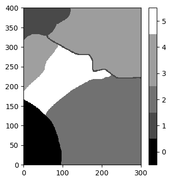
Note that the colors are reordered (i.e. the variable values are reordered).
Dealing with missing value
[33]:
nancol = col[2] # color code of the category "2" in initial image

# Read the image from the initial file, specifying a color to be interpreted as missing value
im_cat_b_x, col_b_x = gn.img.readImage2Drgb(os.path.join(data_dir, f'{fbase}.{ext}'),
                                            categ=True, nancol=nancol, keep_channels=False)

# Show info
print('Same geone images (im_cat_x and im_cat_b_x) ?', gn.img.isImageEqual(im_cat_x, im_cat_b_x))
print('List of colors (rate in [0,1]):', col_b_x)
Same geone images (im_cat_x and im_cat_b_x) ? True
List of colors (rate in [0,1]): [0.         0.61614118 0.28934118 0.44227059 1.        ]
[34]:
# Get RGB(A) colors via a color map
cmap = plt.get_cmap('gray')
col_b_x_rgb = [cmap(c) for c in col_b_x]
col_b_x_rgb
[34]:
[(np.float64(0.0), np.float64(0.0), np.float64(0.0), np.float64(1.0)),
 (np.float64(0.615686274509804),
  np.float64(0.615686274509804),
  np.float64(0.615686274509804),
  np.float64(1.0)),
 (np.float64(0.2901960784313725),
  np.float64(0.2901960784313725),
  np.float64(0.2901960784313725),
  np.float64(1.0)),
 (np.float64(0.44313725490196076),
  np.float64(0.44313725490196076),
  np.float64(0.44313725490196076),
  np.float64(1.0)),
 (np.float64(1.0), np.float64(1.0), np.float64(1.0), np.float64(1.0))]
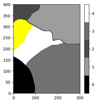
[35]:
# Plot the image with gn.imgplot.drawImage2D
plt.figure(figsize=(4,4))
gn.imgplot.drawImage2D(im_cat_b_x, categ=True, categCol=col_b_x_rgb, categColbad='yellow')
plt.show()
[36]:
# Write image accounting for missing value
out_file = f'{fbase}_b_x_new.{ext}' # output file
f = os.path.join(out_dir, out_file)
gn.img.writeImage2Drgb(f, im_cat_b_x, col=col_b_x_rgb, nancol='yellow') # use RGB(A) colors def. in col_b_x_rgb

# Read the image from the written file (keeping RGB(A) channels) and plot it (recombining the RGB(A) channels)
im_cat_b_x_new, col_b_x_new = gn.img.readImage2Drgb(f, categ=True, nancol='yellow') # keeping channels
print('Same geone images (im_cat_b_x and im_cat_b_x_new) ?', gn.img.isImageEqual(im_cat_b_x, im_cat_b_x_new))

plt.figure(figsize=(4,4))
gn.imgplot.drawImage2D(im_cat_b_x_new, categ=True, categCol=col_b_x_new, categColbad='yellow')
plt.show()
Same geone images (im_cat_b_x and im_cat_b_x_new) ? False
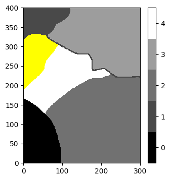
Note that the colors are reordered (i.e. the variable values are reordered).