GEONE - Images interpolation

This notebook introduces some tools to interpolate an image (class geone.img.Img).

Import what is required

import numpy as np
import matplotlib.pyplot as plt
import os

# import package 'geone'
import geone as gn

# Show version of python and version of geone
import sys
print(sys.version_info)
print('geone version: ' + gn.__version__)

sys.version_info(major=3, minor=13, micro=7, releaselevel='final', serial=0)
geone version: 1.3.3

Remark

The matplotlib figures can be visualized in interactive mode:

• %matplotlib notebook: enable interactive mode

• %matplotlib inline: disable interactive mode

Interpolate an image

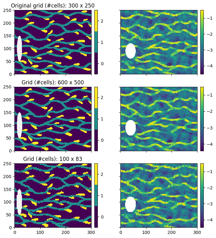
The function geone.img.interpolateImage interpolates (each variable of) an image on a given grid, and returns the result on an output image. This allows for example to make an image finer or coarser. Both categorical and continuous variables are handled. See the example below.

# Read a bivariate 2D image:
# - variable of index 0: categorical
# - variable of index 1: continuous
data_dir = 'data'
filename = os.path.join(data_dir, 'ti_2var.txt')
im = gn.img.readImageTxt(filename)

# Set some undefined value (np.nan)
im.val[0, ((im.xx()-20)/10)**2 + ((im.yy()-100)/50)**2 < 1] = np.nan
im.val[1, ((im.xx()-40)/20)**2 + ((im.yy()-90)/30)**2 < 1] = np.nan

# Refine image
nx_new = 2*im.nx
ny_new = 2*im.ny
im_new = gn.img.interpolateImage(im, nx=nx_new, ny=ny_new, categVar=[True, False])

# Make the image coarser
nx_new_2 = int(im.nx/3)
ny_new_2 = int(im.ny/3)
im_new_2 = gn.img.interpolateImage(im, nx=nx_new_2, ny=ny_new_2, categVar=[True, False])

plt.subplots(3, 2, sharex=True, sharey=True, figsize=(8, 9))

plt.subplot(3, 2, 1)
gn.imgplot.drawImage2D(im, iv=0, categ=True)
plt.title(f'Original grid (#cells): {im.nx} x {im.ny}')

plt.subplot(3, 2, 2)
gn.imgplot.drawImage2D(im, iv=1, categ=False)

plt.subplot(3, 2, 3)
gn.imgplot.drawImage2D(im_new, iv=0, categ=True)
plt.title(f'Grid (#cells): {im_new.nx} x {im_new.ny}')

plt.subplot(3, 2, 4)
gn.imgplot.drawImage2D(im_new, iv=1, categ=False)

plt.subplot(3, 2, 5)
gn.imgplot.drawImage2D(im_new_2, iv=0, categ=True)
plt.title(f'Grid (#cells): {im_new_2.nx} x {im_new_2.ny}')

plt.subplot(3, 2, 6)
gn.imgplot.drawImage2D(im_new_2, iv=1, categ=False)

plt.show()

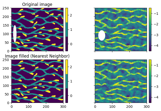
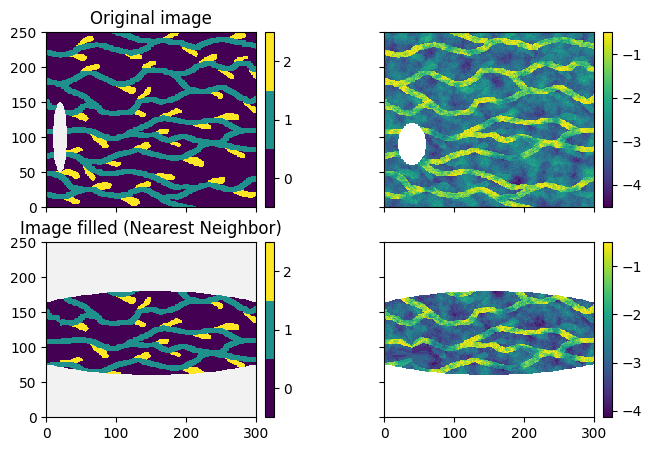
Fill an image with respect to nearest neighbor

The function fill_image_nearest_neighbor is used to fill an image (optionally in an area specified by a mask array). See the doc for more details.

im_filled = gn.img.fill_image_nearest_neighbor(im)

plt.subplots(2, 2, sharex=True, sharey=True, figsize=(8, 5))

plt.subplot(2, 2, 1)
gn.imgplot.drawImage2D(im, iv=0, categ=True)
plt.title(f'Original image')

plt.subplot(2, 2, 2)
gn.imgplot.drawImage2D(im, iv=1, categ=False)

plt.subplot(2, 2, 3)
gn.imgplot.drawImage2D(im_filled, iv=0, categ=True)
plt.title(f'Image filled (Nearest Neighbor)')

plt.subplot(2, 2, 4)
gn.imgplot.drawImage2D(im_filled, iv=1, categ=False)


plt.show()

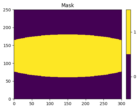
Using a mask

# Define a mask array (True where the filling is applied)
mask_array = ((im.xx()-150)/220)**2 + ((im.yy()-120)/60)**2 < 1

# Show mask area
im_mask = gn.img.Img(nx=im.nx, ny=im.ny, nz=im.nz,
                     sx=im.sx, sy=im.sy, sz=im.sz,
                     ox=im.ox, oy=im.oy, oz=im.oz,
                     nv=1, val=mask_array)

plt.figure(figsize=(5, 5))
gn.imgplot.drawImage2D(im_mask, categ=True)
plt.title(f'Mask')
plt.show()

# Apply filling in mask area
im_filled = gn.img.fill_image_nearest_neighbor(im, mask_array=mask_array)

plt.subplots(2, 2, sharex=True, sharey=True, figsize=(8, 5))

plt.subplot(2, 2, 1)
gn.imgplot.drawImage2D(im, iv=0, categ=True)
plt.title(f'Original image')

plt.subplot(2, 2, 2)
gn.imgplot.drawImage2D(im, iv=1, categ=False)

plt.subplot(2, 2, 3)
gn.imgplot.drawImage2D(im_filled, iv=0, categ=True)
plt.title(f'Image filled (Nearest Neighbor)')

plt.subplot(2, 2, 4)
gn.imgplot.drawImage2D(im_filled, iv=1, categ=False)


plt.show()

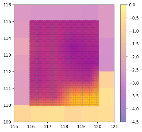
Interpolator (function) from an image

The class Img_interp_func defines an interpolator from one variable defined in an image. See the doc for more details.

# Get interpolator function from the variable of index 1 of the image im within the slice iz=0
interp = gn.img.Img_interp_func(im, ind=1, iz=0)

# Set some points within the grid
xmin, xmax = 116, 120
ymin, ymax = 110, 115
mx, my = 30, 50
x = np.linspace(xmin, xmax, mx)
y = np.linspace(ymin, ymax, my)
yy, xx = np.meshgrid(y, x, indexing='ij')
points = np.array((xx.reshape(-1), yy.reshape(-1))).T

# Get the values via the interpolator
v = interp(points)

# Plot underlying image (from which the interpolator is defined) and the points
cmap='plasma'
vmin, vmax = -4.5, 0.

plt.figure(figsize=(8,5))
gn.imgplot.drawImage2D(im, iv=1, categ=False, cmap=cmap, vmin=vmin, vmax=vmax, alpha=.5)
plot = plt.scatter(points[:,0], points[:,1], c=v, cmap=cmap, vmin=vmin, vmax=vmax,
                   edgecolors='black', linewidths=.1)
plt.xlim(xmin-1, xmax+1)
plt.ylim(ymin-1, ymax+1)
plt.show()

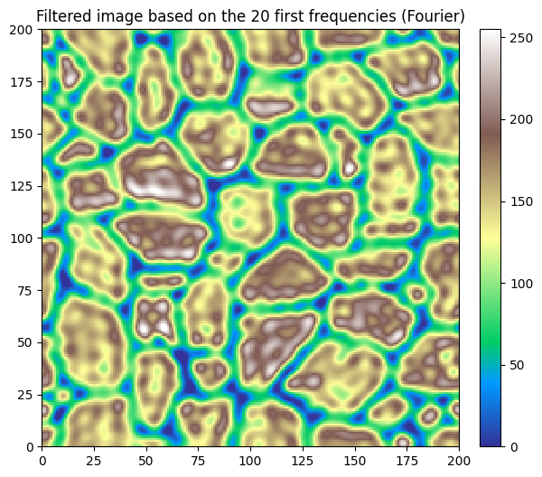
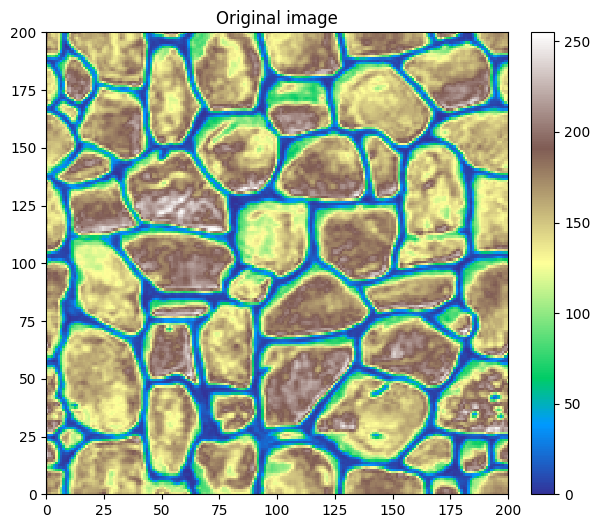
Filtering signal (Fourier)

The function geone.tools.filter_signal allows to filter a signal (numpy.nd-array) based on Fourier transforms. See the doc for more details.

A basic illustration is proposed below on a 2D continuous image (signal).

# Read file
data_dir = 'data'
filename = os.path.join(data_dir, 'tiContinuous.txt')
im = gn.img.readImageTxt(filename)

# Color settings
cmap='terrain'
vmin, vmax = im.vmin(), im.vmax()

# Plot
plt.figure(figsize=(12,6))
gn.imgplot.drawImage2D(im, cmap=cmap, vmin=vmin, vmax=vmax)
plt.title('Original image')
plt.show()

# Extract the numpy 2d-array of the image
s = im.val[0, 0] # original signal

# Filter the signal based on the `n` first positive frequencies
n = 20
s_filter = gn.tools.filter_signal(s, n=n)

# Set the filtered image
im_filter = gn.img.copyImg(im)
im_filter.set_var(s_filter, ind=0)
# im_filter.val[0, 0] = s_filter # equiv.

# Plot
plt.figure(figsize=(12,6))
gn.imgplot.drawImage2D(im_filter, cmap=cmap, vmin=vmin, vmax=vmax)
plt.title(f'Filtered image based on the {n} first frequencies (Fourier)')
plt.show()