GEONE - DEESSE - Basics

Main points addressed

launching deesse
simple deesse simulations of a categorical variable, with hard data points
basic statistics on the results
deesse simulation using pyramids (multi-resolution)

Import what is required

[1]:

import numpy as np
import matplotlib.pyplot as plt
import time
import os

# import package 'geone'
import geone as gn

[2]:

# Show version of python and version of geone
import sys
print(sys.version_info)
print('geone version: ' + gn.__version__)

sys.version_info(major=3, minor=13, micro=7, releaselevel='final', serial=0)
geone version: 1.3.0

Remark

The matplotlib figures can be visualized in interactive mode:

%matplotlib notebook: enable interactive mode
%matplotlib inline: disable interactive mode

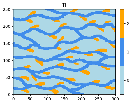
Training image (TI)

Read the file ti.txt using the function geone.img.readImageTxt (see jupyter notebook ex_a_01_image_and_pointset.ipynb for details).

[3]:

data_dir = 'data' # directory containing the training image file
filename = os.path.join(data_dir, 'ti.txt')
ti = gn.img.readImageTxt(filename)
ti

[3]:

*** Img object ***
name = 'data/ti.txt'
(nx, ny, nz) = (300, 250, 1) # number of cells along each axis
(sx, sy, sz) = (1.0, 1.0, 1.0) # cell size (spacing) along each axis
(ox, oy, oz) = (0.0, 0.0, 0.0) # origin (coordinates of bottom-lower-left corner)
nv = 1  # number of variable(s)
varname = [np.str_('code')]
val: (1, 1, 250, 300)-array
*****

[4]:

# Values taken in ti
ti.get_unique()

[4]:

array([0., 1., 2.])

Plot the image using the function geone.imgplot.drawImage2D (see jupyter notebook ex_a_01_image_and_pointset.ipynb for details).

[5]:

# Define category values and colors
categ_val = [0, 1, 2]
categ_col = ['lightblue', [x/255. for x in ( 65, 141, 235)], 'orange']

plt.figure(figsize=(5,5))
gn.imgplot.drawImage2D(ti, categ=True, categVal=categ_val, categCol=categ_col)
plt.title('TI')
plt.show()

../_images/notebooks_ex_deesse_01_basics_9_0.png

Simulation grid

Define the simulation grid (number of cells in each direction, cell unit, origin).

[6]:

nx, ny, nz = 100, 100, 1         # number of cells
sx, sy, sz = ti.sx, ti.sy, ti.sz # cell unit
ox, oy, oz = 0.0, 0.0, 0.0       # origin (corner of the "first" grid cell)

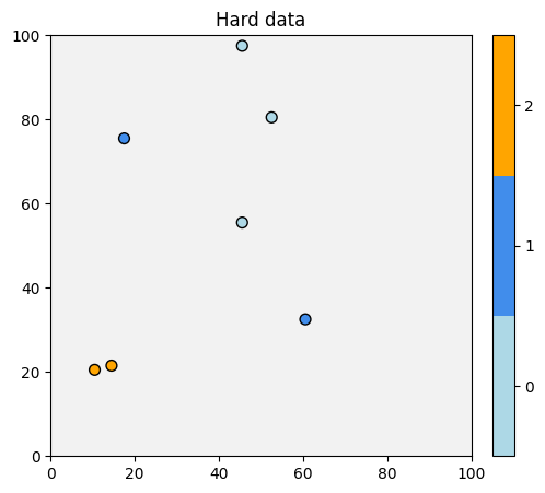
Hard data (point set)

Read the file hd.txt using the function geone.img.readPointSetTxt (see jupyter notebook ex_a_01_image_and_pointset.ipynb for details).

[7]:

data_dir = 'data'
filename = os.path.join(data_dir, 'hd.txt')
hd = gn.img.readPointSetTxt(filename)
hd

[7]:

*** PointSet object ***
name = ''
npt = 7 # number of point(s)
nv = 4  # number of variable(s) (including coordinates)
varname = [np.str_('X'), np.str_('Y'), np.str_('Z'), np.str_('code')]
val: (4, 7)-array
*****

[8]:

hd.val

[8]:

array([[10.5, 14.5, 60.5, 45.5, 17.5, 52.5, 45.5],
       [20.5, 21.5, 32.5, 55.5, 75.5, 80.5, 97.5],
       [ 0. ,  0. ,  0. ,  0. ,  0. ,  0. ,  0. ],
       [ 2. ,  2. ,  1. ,  0. ,  1. ,  0. ,  0. ]])

The array hd.val contains:

hd.val[0]: $x$ coordinates of the points
hd.val[1]: $y$ coordinates of the points
hd.val[2]: $z$ coordinates of the points
hd.val[3]: value of the next variable (stored in the point set)

Plot the hard data points in the simulation grid.

[9]:

# Get the colors for values of the variable of index 3 in the point set,
# according to the color settings used for the TI
hd_col = gn.imgplot.get_colors_from_values(hd.val[3], categ=True, categVal=categ_val, categCol=categ_col)

# Set an image with simulation grid geometry defined above, and no variable
im_empty = gn.img.Img(nx, ny, nz, sx, sy, sz, ox, oy, oz, nv=0)

# Plot
plt.figure(figsize=(8,5))

# Plot empty simulation grid and specify colors
gn.imgplot.drawImage2D(im_empty, categ=True, categVal=categ_val, categCol=categ_col)

# Add hard data points
plt.scatter(hd.x(), hd.y(), marker='o', s=50, color=hd_col, edgecolors='black', linewidths=1)

plt.title('Hard data')
plt.show()

../_images/notebooks_ex_deesse_01_basics_17_0.png

Input structure for deesse (class `geone.deesseinterface.DeesseInput`)

The variable name for the hard data (in hd.varname) and for the simulated variable (keyword argument varname below) should be the same, otherwise, the hard data will be ignored. Moreover, the hard data locations should be in the simulation grid, which is described by its dimensions (number of cells) in each direction, the cell unit in each direction, and the origin (the corner of the grid cell with the minimal x, y, z coordinates). Hard data points out of the simulation grid are ignored.

The hard data can be passed to deesse through a point set, i.e. a class geone.img.PointSet (keyword argument dataPointSet, as below) or through an image, i.e. a class geone.img.Img (keyword argument dataImage, not illustrated here), and can contain missing (uninformed) data (nan).

The type of distance for computing the dissimilarity between patterns is controlled by the keyword argument distanceType:

0 or 'categorical': proportion of non-matching nodes (default)
1 or 'continuous': $L_1$ distance
2: $L_2$ distance
3: $L_p$ distance (requires real positive parameter p given in parameter powerLpDistance)
4 : $L_\infty$ distance

[10]:

nreal = 20
deesse_input = gn.deesseinterface.DeesseInput(
    nx=nx, ny=ny, nz=nz,        # dimension of the simulation grid (number of cells)
    sx=sx, sy=sy, sz=sz,        # cells units in the simulation grid
    ox=ox, oy=oy, oz=oz,        # origin of the simulation grid
    nv=1, varname='code',       # number of variable(s), name of the variable(s)
    TI=ti,                      # TI (class gn.deesseinterface.Img)
    dataPointSet=hd,            # hard data (optional)
    distanceType='categorical', # distance type: proportion of mismatching nodes (categorical var., default)
    #conditioningWeightFactor=10.,  # put more weight to conditioning data (if needed)
    nneighboringNode=24,        # max. number of neighbors (for the patterns)
    distanceThreshold=0.05,     # acceptation threshold (for distance between patterns)
    maxScanFraction=0.25,       # max. scanned fraction of the TI (for simulation of each cell)
    npostProcessingPathMax=1,   # number of post-processing path(s)
    seed=444,                   # seed (initialization of the random number generator)
    nrealization=nreal)         # number of realization(s)

Launching deesse

Launch deesse: function `geone.deesseinterface.deesseRun`

The function geone.deesseinterface.deesseRun launches deesse. The code runs in parallel (based on OpenMP). The number of threads used can be specified by the keyword argument nthreads. Specifying a number -n, negative or zero, means that the total number of cpus of the system (retrieved by os.cpu_count()) except n (but at least one) will be used. By default: nthreads=-1.

Remark: the keyword argument verbose allows to control what is displayed, verbose=0: minimal display, verbose=1: only errors (if any), verbose=2 (default): version and warning(s) encountered, verbose=3: version, progress, and warning(s) encountered. Note that due to buffering, progress might not be displayed immediately and then could be useless.

[11]:

t1 = time.time() # start time
deesse_output = gn.deesseinterface.deesseRun(deesse_input, nthreads=8)
t2 = time.time() # end time
print(f'Elapsed time: {t2-t1:.2g} sec')

deesseRun: DeeSse running... [VERSION 3.2 / BUILD NUMBER 20230914 / OpenMP 8 thread(s)]
deesseRun: DeeSse run complete
Elapsed time: 2.3 sec

Launch deesse on multiple processes: function `geone.deesseinterface.deesseRun_mp`

The function geone.deesseinterface.deesseRun_mp launches deesse on multiple processes.

Specifying the number of processes, nproc, and the number of threads per process, nthreads_per_proc, this function will run nproc parallel processes (parallel calls of function geone.deesseinterface.deesseRun), each one using nthreads_per_proc threads. The ensemble of realizations (specified by nreal) is distributed in a balanced way over the process(es).

In terms of resources, this implies the use of nproc $\cdot$ nthreads_per_proc cpu(s).

First, the number of process(es) is set. A negative number (or zero) (by default nproc=-1), nproc = -n $\leqslant$ 0, can be specified to use the total number of cpu(s) of the system except n; nproc is finally at maximum equal to nreal but at least 1 by applying:

if nproc $\geqslant$ 1, then nproc = max(min(nproc, nreal), 1) is used
if nproc = -n $\leqslant$ 0, then nproc = max(min(nmax - n, nreal), 1) is used, where nmax is the total number of cpu(s) of the system (retrieved by os.cpu_count())

Then, the number of threads per process is set. If nthreads_per_proc = -n <= 0 (by default nthreads_per_proc = -1), nthreads_per_proc is set to the maximal integer (but at least 1) such that nproc $\cdot$ nthreads_per_proc $\leqslant$ nmax - n, where nmax is the total number of cpu(s) of the system (retrieved by multiprocessing.cpu_count()).

These parameters must be set cautiously, because the product nproc $\cdot$ nthreads_per_proc can exceed nmax, the total number of cpu(s) of the system.

Remark: the keyword argument verbose allows to control what is displayed, verbose=0: minimal display, verbose=1: only errors and notes (if any), verbose=2 (default): version and warning(s) encountered.

Note about `multiprocessing`

Some functions uses multiprocessing with each process running on multi-threads (OpenMP in pre-compiled C libraries). If such a function blocks, this might be due to the “start method” of multiprocessing, which is set to ‘fork’ by default on Linux. Setting “start method” to ‘spawn’ might solve this issue, at the cost of performance. Or, to keep better performance, “start method” can be let (set) to ‘fork’, and in function allowing to specify the number of process(es) nproc and the number of thread(s) per process nthreads_per_proc, use set-up such that nproc=1 or nthreads_per_proc=1.

Important: if needed, “start method” of multiprocessing must be set at START OF THE PYTHON SESSION, i.e. before running any multiprocessing task, with

import multiprocessing
multiprocessing.set_start_method(start_method)

where start_method is a string (e.g. ‘spawn’, ‘fork’); or this can be forced by using the keyword argument force=True. Note that multiprocessing.get_start_method() returns the “start method”.

[12]:

t1 = time.time() # start time
deesse_output2 = gn.deesseinterface.deesseRun_mp(deesse_input, nproc=4, nthreads_per_proc=4)
t2 = time.time() # end time
print(f'Elapsed time: {t2-t1:.2g} sec')

deesseRun_mp: DeeSse running on 4 process(es)... [VERSION 3.2 / BUILD NUMBER 20230914 / OpenMP 4 thread(s)]
deesseRun_mp: DeeSse run complete (all process(es))
Elapsed time: 1.3 sec

Computational resources - Important remark

Although some default values are proposed for nthreads, nproc, nthreads_per_proc, it is strongly recommended to specify these parameters controlling the computational resources; a few tests on the machine used allows to select a good set-up.

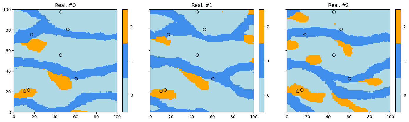
Retrieve the results (and display)

The function geone.deesseinterface.deesseRun (or geone.deesseinterface.deesseRun_mp) returns a dictionary deesse_output containing the keys: 'sim', 'nwarnings', 'warnings' (plus other ones).

The realizations are stored in deesse_output['sim'], a 1-dimensional array of images (class geone.img.Img) of size deesse_input.nrealization, deesse_output['sim'][i] being the i-th realization.

The total number of warning(s) encountered during the simulation are stored in deesse_output['nwarning'] (int), and all the distinct warning messages are stored in deesse_output['warnings'] (a list, possibly empty).

Moreover, additional information can be retrieved in output: the simulation path map (index in the simulation path), the error map (error for the retained candidate), the TI grid node index map (index of the grid node of the retained candidate in the TI) and the TI index map (index of the TI used (makes sense if number of TIs, deesse_input.nTI, is greater than 1)). These maps are images with the simulation grid as grid (support), and can be retrieved in output in deesse_output['path'], deesse_output['error'], deesse_output['tiGridNode'] and deesse_output['tiIndex'] respectively. However, these ouputs are set to None by default. See jupyter notebook ex_deesse_02_additional_outputs_and_simulation_paths.ipynb for illustrations.

[13]:

# deesse_output and deesse_output2 above give same results
ok = np.all([np.all(im.val == im2.val) for im, im2 in zip(deesse_output['sim'], deesse_output2['sim'])])
# # or equivalently:
# ok = np.all([np.all(deesse_output['sim'][i].val == deesse_output2['sim'][i].val) for i in range(nreal)])

print(f'Identical result: {ok}') # should be True

Identical result: True

[14]:

# Total number of warning(s), and warning messages
deesse_output['nwarning'], deesse_output['warnings']

[14]:

(0, [])

[15]:

# Retrieve the realizations
sim = deesse_output['sim']

# Display
# -------
# Get colors for hard data (according to variable of index 3 in the point set, and color settings)
hd_col = gn.imgplot.get_colors_from_values(hd.val[3], categ=True, categVal=categ_val, categCol=categ_col)
# # or equivalently:
# import matplotlib.colors
# hd_col=[matplotlib.colors.to_rgba(categ_col[int(v)]) for v in hd.val[3]] # colors (converted to 'rgba')
#                                                                          # of hard data points

plt.subplots(1, 3, figsize=(17,5), sharey=True)
for i in range(3):
    plt.subplot(1, 3, i+1) # select next sub-plot

    # Plot realization #i
    gn.imgplot.drawImage2D(sim[i], categ=True, categVal=categ_val, categCol=categ_col)
    # Add hard data points
    plt.scatter(hd.x(), hd.y(), marker='o', s=50, color=hd_col, edgecolors='black', linewidths=1)

    plt.title(f'Real. #{i}')

plt.show()

../_images/notebooks_ex_deesse_01_basics_29_0.png

Do some statistics on the realizations

The function geone.img.imageCategProp(im, categ) allows to compute the pixel-wise proportions of given categories in the list categ over all the variables of the image im. First, an image with nreal variables, each one corresponding to one realization, is defined (from the array of realizations) using the function geone.img.gatherImages.

Alternatively, the function geone.img.imageListCategProp(im_list, categ, ind) can be used directly to compute the pixel-wise proportions of given categories in the list categ over the variable of index ind of all the images in the list im_list.

[16]:

# Gather the nreal realizations into one image
all_sim = gn.img.gatherImages(sim) # all_sim is one image with nreal variables

# Do statistics over all the realizations: compute the pixel-wise proportion for the given categories
all_sim_stats = gn.img.imageCategProp(all_sim, categ_val)

[17]:

# Equivalently:
all_sim_stats2 = gn.img.imageListCategProp(sim, categ_val)

print("Same result ?", gn.img.isImageEqual(all_sim_stats, all_sim_stats2)) # should be True

Same result ? True

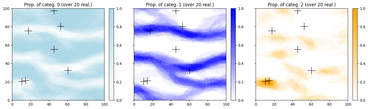
Plot the results.

[18]:

prop_col=['lightblue', 'blue', 'orange'] # colors for the proportion maps
cmap = [gn.customcolors.custom_cmap(['white', c]) for c in prop_col]

# Display
plt.subplots(1, 3, figsize=(17,5), sharey=True)
for i in range(3):
    plt.subplot(1, 3, i+1) # select next sub-plot
    gn.imgplot.drawImage2D(all_sim_stats, iv=i, cmap=cmap[i],
                           title=f'Prop. of categ. {i} (over {nreal} real.)')
    plt.plot(hd.x(), hd.y(), '+', markersize=20, c='black') # add hard data points
plt.show()

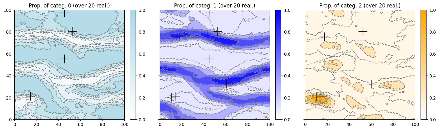
../_images/notebooks_ex_deesse_01_basics_34_0.png

[19]:

# Display with other styles (level (iso-value) curves)
plt.subplots(1, 3, figsize=(17,5), sharey=True)
for i in range(3):
    plt.subplot(1, 3, i+1) # select next sub-plot
    gn.imgplot.drawImage2D(all_sim_stats, iv=i, cmap=cmap[i],
                           contourf=True, # fill between level (iso-value) curves
                           contour=True,  # draw level (iso-value) curves
                           levels=5, #levels=np.arange(0.0, 1.1, 0.2), # specify levels (iso-values)
                           contour_clabel=True, # draw value on level curves
                           contour_kwargs={'linestyles':'dashed', 'colors':'gray'},
                           contour_clabel_kwargs={'fontsize':10, 'inline':1},
                           title=f'Prop. of categ. {i} (over {nreal} real.)')
    plt.plot(hd.x(), hd.y(), '+', markersize=20, c='black') # add hard data points
plt.show()

../_images/notebooks_ex_deesse_01_basics_35_0.png

Simulations using pyramids

Enabling pyramids implies multi-resolution simulations, which can help to better reproduce the spatial structures. It consists in considering lower resolutions of the TI and the simulation grid.

See jupyter notebook ex_deesse_16_advanced_use_of_pyramids.ipynb for more details about pyramids.

Parameters for pyramids

Class `geone.deesseinterface.PyramidGeneralParameters` and class `geone.deesseinterface.PyramidParameters`

Using pyramids requires to define:

General parameters (class geone.deesseinterface.PyramidGeneralParameters):
- the number of pyramid levels (npyramidLevel) additional to the original simulation grid
- the reduction factors along each axis direction (kx, ky, kz, list of length npyramidLevel): the integers kx[i], ky[i], kz[i] are these factors between the level i and the level i+1 (the number of cells in each direction are respectively divided by these factors), the simulation grid being the level 0, and the lowest resolution being the level npyramidLevel. (A factor set to zero means that no reduction is made along the corresponding direction.)
Parameters for each variable (one variable in this example (univariate simulation)):
- the number of levels (nlevel, should be equal to npyramidLevel above)
- the type of pyramid (pyramidType), which depends on the type of the variable

Note: in the example below, the pyramid type is set to categorical_auto: one pyramid for the indicator variable of each category except one is built and used.

Note that simulation results in the pyramid (additional levels) can be retrieved in ouput; they are stored in the output dictionnary returned by a deesse simulation under the key 'sim_pyramid'. This output is set to None by default. See jupyter notebook ex_deesse_16_advanced_use_of_pyramids.ipynb for illustrations.

[20]:

pyrGenParams = gn.deesseinterface.PyramidGeneralParameters(
    npyramidLevel=2,                 # number of pyramid levels, additional to the simulation grid
    kx=[2, 2], ky=[2, 2], kz=[0, 0]  # reduction factors from one level to the next one
                                     #    (kz=[0, 0]: do not apply reduction along z axis)
)

pyrParams = gn.deesseinterface.PyramidParameters(
    nlevel=2,                      # number of levels
    pyramidType='categorical_auto' # type of pyramid (accordingly to categorical variable in this example)
)

Fill the input structure for deesse and launch deesse

[21]:

deesse_input = gn.deesseinterface.DeesseInput(
    nx=nx, ny=ny, nz=nz,
    sx=sx, sy=sy, sz=sz,
    ox=ox, oy=oy, oz=oz,
    nv=1, varname='code',
    TI=ti,
    dataPointSet=hd,
    distanceType='categorical',
    nneighboringNode=24,
    distanceThreshold=0.05,
    maxScanFraction=0.25,
    pyramidGeneralParameters=pyrGenParams, # set pyramid general parameters
    pyramidParameters=pyrParams,           # set pyramid parameters for each variable
    npostProcessingPathMax=1,
    seed=444,
    nrealization=nreal)

# Run deesse
t1 = time.time() # start time
deesse_output = gn.deesseinterface.deesseRun(deesse_input, nthreads=8)
t2 = time.time() # end time
print(f'Elapsed time: {t2-t1:.2g} sec')

deesseRun: DeeSse running... [VERSION 3.2 / BUILD NUMBER 20230914 / OpenMP 8 thread(s)]
deesseRun: DeeSse run complete
Elapsed time: 4.4 sec

[22]:

# Alternatively, using multiple processes
t1 = time.time() # start time
deesse_output2 = gn.deesseinterface.deesseRun_mp(deesse_input, nproc=4, nthreads_per_proc=4)
t2 = time.time() # end time
print(f'Elapsed time: {t2-t1:.2g} sec')

deesseRun_mp: DeeSse running on 4 process(es)... [VERSION 3.2 / BUILD NUMBER 20230914 / OpenMP 4 thread(s)]
deesseRun_mp: DeeSse run complete (all process(es))
Elapsed time: 2.4 sec

[23]:

# deesse_output and deesse_output2 above give same results
ok = np.all([np.all(im.val == im2.val) for im, im2 in zip(deesse_output['sim'], deesse_output2['sim'])])
## equiv.
#ok = np.all([np.all(deesse_output['sim'][i].val == deesse_output2['sim'][i].val) for i in range(nreal)])
print(f'Identical result: {ok}') # should be True

Identical result: True

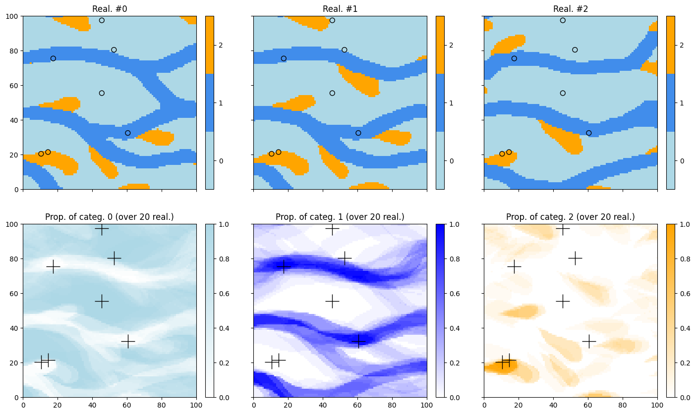
Results

[24]:

# Retrieve the realizations
sim = deesse_output['sim']

# Gather the nreal realizations into one image
all_sim = gn.img.gatherImages(sim) # all_sim is one image with nreal variables

# Do statistics over all the realizations: compute the pixel-wise proportion for the given categories
all_sim_stats = gn.img.imageCategProp(all_sim, [0, 1, 2])

# Display
plt.subplots(2, 3, figsize=(17,10), sharex=True, sharey=True)
for i in range(3):
    plt.subplot(2, 3, i+1) # select next sub-plot
    gn.imgplot.drawImage2D(sim[i], categ=True, categVal=categ_val, categCol=categ_col, title=f'Real. #{i}')
    plt.scatter(hd.x(), hd.y(), marker='o', s=50,
                color=hd_col, edgecolors='black', linewidths=1) # add hard data points
for i in range(3):
    plt.subplot(2, 3, i+4) # select next sub-plot
    gn.imgplot.drawImage2D(all_sim_stats, iv=i, cmap=cmap[i],
                           title=f'Prop. of categ. {i} (over {nreal} real.)')
    plt.plot(hd.x(), hd.y(), '+', c='black', markersize=20) # add hard data points
plt.show()

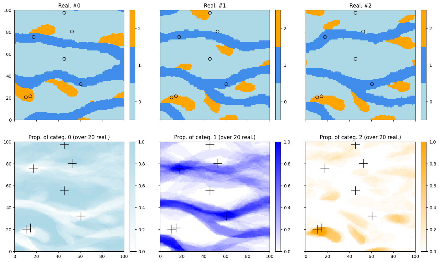
../_images/notebooks_ex_deesse_01_basics_44_0.png

Simulations using pyramids (2)

Here the pyramid type is set to categorical_to_continuous: the pyramid is built for one continuous variable derived from the categorical variable (accounting for the connections between adjacent nodes).

[25]:

# Deesse input
pyrParams = gn.deesseinterface.PyramidParameters(
    nlevel=2,
    pyramidType='categorical_to_continuous' # type of pyramid (accordingly to categ. variable in this example)
)

deesse_input = gn.deesseinterface.DeesseInput(
    nx=nx, ny=ny, nz=nz,
    sx=sx, sy=sy, sz=sz,
    ox=ox, oy=oy, oz=oz,
    nv=1, varname='code',
    TI=ti,
    dataPointSet=hd,
    distanceType='categorical',
    nneighboringNode=24,
    distanceThreshold=0.05,
    maxScanFraction=0.25,
    pyramidGeneralParameters=pyrGenParams,
    pyramidParameters=pyrParams,
    npostProcessingPathMax=1,
    seed=444,
    nrealization=nreal)

# Run deesse
t1 = time.time() # start time
deesse_output = gn.deesseinterface.deesseRun(deesse_input, nthreads=8)
t2 = time.time() # end time
print(f'Elapsed time: {t2-t1:.2g} sec')

deesseRun: DeeSse running... [VERSION 3.2 / BUILD NUMBER 20230914 / OpenMP 8 thread(s)]
deesseRun: DeeSse run complete
Elapsed time: 1.9 sec

[26]:

# Alternatively, using multiple processes
t1 = time.time() # start time
deesse_output2 = gn.deesseinterface.deesseRun_mp(deesse_input, nproc=4, nthreads_per_proc=4)
t2 = time.time() # end time
print(f'Elapsed time: {t2-t1:.2g} sec')

deesseRun_mp: DeeSse running on 4 process(es)... [VERSION 3.2 / BUILD NUMBER 20230914 / OpenMP 4 thread(s)]
deesseRun_mp: DeeSse run complete (all process(es))
Elapsed time: 0.98 sec

[27]:

# deesse_output and deesse_output2 above give same results
ok = np.all([np.all(im.val == im2.val) for im, im2 in zip(deesse_output['sim'], deesse_output2['sim'])])
#ok = np.all([np.all(deesse_output['sim'][i].val == deesse_output2['sim'][i].val) for i in range(nreal)]) # equiv.
print(f'Identical result: {ok}') # should be True

Identical result: True

Results

[28]:

# Retrieve the realizations
sim = deesse_output['sim']

# Gather the nreal realizations into one image
all_sim = gn.img.gatherImages(sim) # all_sim is one image with nreal variables

# Do statistics over all the realizations: compute the pixel-wise proportion for the given categories
all_sim_stats = gn.img.imageCategProp(all_sim, [0, 1, 2])

# Display
plt.subplots(2, 3, figsize=(17,10), sharex=True, sharey=True)
for i in range(3):
    plt.subplot(2, 3, i+1) # select next sub-plot
    gn.imgplot.drawImage2D(sim[i], categ=True, categVal=categ_val, categCol=categ_col, title=f'Real. #{i}')
    plt.scatter(hd.x(), hd.y(), marker='o', s=50,
                color=hd_col, edgecolors='black', linewidths=1) # add hard data points
for i in range(3):
    plt.subplot(2, 3, i+4) # select next sub-plot
    gn.imgplot.drawImage2D(all_sim_stats, iv=i, cmap=cmap[i],
                           title=f'Prop. of categ. {i} (over {nreal} real.)')
    plt.plot(hd.x(), hd.y(), '+', c='black', markersize=20) # add hard data points
plt.show()

../_images/notebooks_ex_deesse_01_basics_50_0.png

3D example

[29]:

import pyvista as pv
pv.set_jupyter_backend('static') # to get static plots within the jupyter notebook

3D Training image

Load from the file ‘ti_3d.txt’.

[30]:

data_dir = 'data'
filename = os.path.join(data_dir, 'ti_3d.txt')
ti3d = gn.img.readImageTxt(filename)
ti3d

[30]:

*** Img object ***
name = 'data/ti_3d.txt'
(nx, ny, nz) = (100, 90, 80) # number of cells along each axis
(sx, sy, sz) = (1.0, 1.0, 1.0) # cell size (spacing) along each axis
(ox, oy, oz) = (0.5, 0.5, 0.5) # origin (coordinates of bottom-lower-left corner)
nv = 1  # number of variable(s)
varname = [np.str_('data')]
val: (1, 80, 90, 100)-array
*****

3D plots

The following functions can be used:

geone.imgplot3d.drawImage3D_volume: 3D plot of volumes (smooth interpolation on the vertex of the cells)
geone.imgplot3d.drawImage3D_surface: 3D plot of surfaces (values at cells are plotted)
geone.imgplot3d.drawImage3D_slice: 3D plot of slices (planes) (See jupyter notebook ex_a_01_image_and_pointset.ipynb for details.)

Plot in an interactive figure or inline according to the “Plotter”: pp = pv.Plotter(notebook=False) or pp = pv.Plotter().

[31]:

# Plot "interactive in pop-up window" or "inline" (comment the undesired one) ...
# ... interactive
#pp = pv.Plotter(notebook=False)
# ... inline
pp = pv.Plotter()
gn.imgplot3d.drawImage3D_volume(ti3d, plotter=pp, scalar_bar_kwargs={'vertical':True}, text='TI')
pp.show()

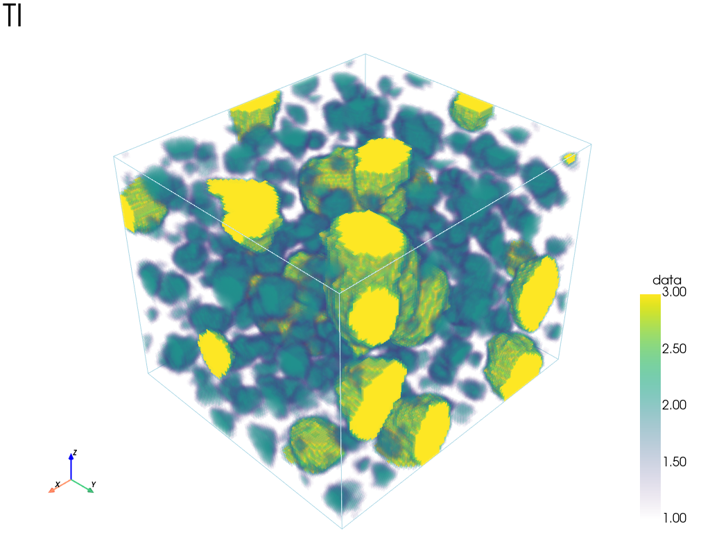
../_images/notebooks_ex_deesse_01_basics_57_0.png

Customize the plot (categorical variable).

[32]:

facies = ti3d.get_unique()
facies

[32]:

array([1., 2., 3.])

[33]:

# Customization of the output:
#    - set mode in "categorical variable" (categ=True), and
#        - specify list of category values (categVal)
#        - specify color for each category value (categCol)
#        - specify which categories are "active" for display (categActive)
#    - set title for the scalar bar
#    - ...
categVal = [1, 2, 3] # list of category values / facies
categCol = ['pink', 'purple', 'yellow'] # colors for each category / facies

# Plot "interactive in pop-up window" or "inline" (comment the undesired one) ...
# ... interactive
#pp = pv.Plotter(notebook=False)
# ... inline
pp = pv.Plotter()
gn.imgplot3d.drawImage3D_surface(
    ti3d,
    plotter=pp, categ=True, categVal=categVal, categCol=categCol,
    categActive=[False, True, True], # display only category value (in categVal) with True
    alpha=1.0, # transparency (alpha channel)
    scalar_bar_kwargs={'title':'facies', 'title_font_size':20, 'vertical':True},
    text='TI'
)
pp.show()

../_images/notebooks_ex_deesse_01_basics_60_0.png

3D Simulation grid

Define the simulation grid (number of cells in each direction, cell unit, origin).

[34]:

nx, ny, nz = 60, 60, 60          # number of cells
sx, sy, sz = ti.sx, ti.sy, ti.sz # cell unit
ox, oy, oz = 0.0, 0.0, 0.0       # origin (corner of the "first" grid cell)

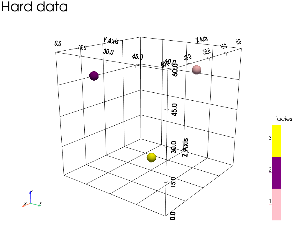
Hard data (point set)

Set some conditioning data.

[35]:

npt = 3 # number of points
nv = 4  # number of variables including x, y, z coordinates
varname = ['x', 'y', 'z', 'code'] # list of variable names
v = np.array([
    [ 15.5,  45.5, 50.5, 1], # x, y, z, code: 1st point
    [ 47.5,  10.5, 48.5, 2], # ...
    [ 27.5,  28.5,  5.5, 3]
    ]).T # variable values: (nv, npt)-array
hd = gn.img.PointSet(npt=npt, nv=nv, varname=varname, val=v)

Plot the hard data points in the simulation grid.

[36]:

# Get colors for hard data (according to variable of index 3 in the point set, and color settings)
hd_col = gn.imgplot.get_colors_from_values(hd.val[3], categ=True, categVal=categVal, categCol=categCol)

# Set points to be plotted
hd_points = pv.PolyData(hd.val[:3].T) # position of the points
hd_points['colors'] = hd_col # colors for the points

# Set an image with simulation grid geometry defined above, and no variable
im_empty = gn.img.Img(nx, ny, nz, sx, sy, sz, ox, oy, oz, nv=0)

# Plot "interactive in pop-up window" or "inline" (comment the undesired one) ...
# ... interactive
#pp = pv.Plotter(notebook=False)
# ... inline
pp = pv.Plotter()

# Plot empty simulation grid and specify colors
gn.imgplot3d.drawImage3D_empty_grid(
    im_empty,
    plotter=pp,
    categ=True, categVal=categVal, categCol=categCol,
    show_bounds=True, bounds_kwargs={'grid':True},
    scalar_bar_kwargs={'title':'facies', 'title_font_size':20, 'vertical':True},
    text='Hard data'
)

# Add hard data points
pp.add_mesh(hd_points, rgb=True, point_size=32., render_points_as_spheres=True) # add data points

# Define cpos by first plotting interactively and then retrieving cpos (pp.show(return_cpos=True)
cpos = [(182.45555265062882, 144.55482888484926, 92.77455190519737),
        (30.0, 30.0, 30.0),
        (-0.24740542241904603, -0.19124554011188336, 0.9498503568167818)]
pp.show(cpos=cpos)

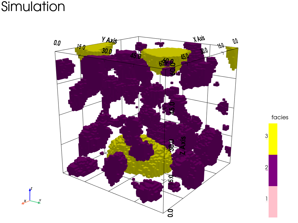
../_images/notebooks_ex_deesse_01_basics_66_0.png

Do a conditional simulation with deesse (3D, with pyramids)

[37]:

# Set input for deesse
pyrGenParams = gn.deesseinterface.PyramidGeneralParameters(
    npyramidLevel=2,
    kx=[2, 2], ky=[2, 2], kz=[2, 2]
)

pyrParams = gn.deesseinterface.PyramidParameters(
    nlevel=2,
    pyramidType='categorical_auto'
)

nreal = 1

deesse_input = gn.deesseinterface.DeesseInput(
    nx=nx, ny=ny, nz=nz,
    sx=sx, sy=sy, sz=sz,
    ox=ox, oy=oy, oz=oz,
    nv=1, varname='code',
    TI=ti3d,
    dataPointSet=hd,
    nneighboringNode=24,
    distanceThreshold=0.02,
    maxScanFraction=0.02,
    pyramidGeneralParameters=pyrGenParams,
    pyramidParameters=pyrParams,
    npostProcessingPathMax=1,
    seed=444,
    nrealization=nreal)

# Run deesse
t1 = time.time() # start time
deesse_output = gn.deesseinterface.deesseRun(deesse_input, nthreads=8)
t2 = time.time() # end time
print(f'Elapsed time: {t2-t1:.2g} sec')

deesseRun: DeeSse running... [VERSION 3.2 / BUILD NUMBER 20230914 / OpenMP 8 thread(s)]
deesseRun: DeeSse run complete
Elapsed time: 13 sec

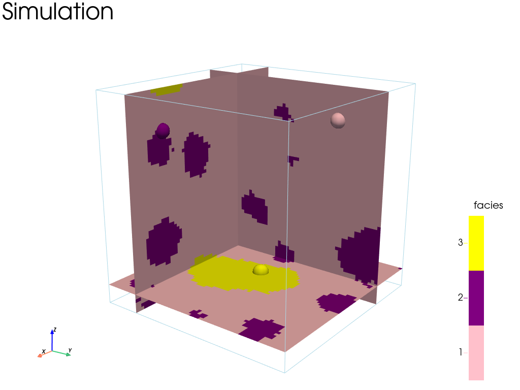
Plot the results

[38]:

# Retrieve the realization
sim = deesse_output['sim']

# Plot "interactive in pop-up window" or "inline" (comment the undesired one) ...
# ... interactive
#pp = pv.Plotter(notebook=False)
# ... inline
pp = pv.Plotter()
gn.imgplot3d.drawImage3D_surface(sim[0], plotter=pp,
    categ=True,
    categVal=categVal,
    categCol=categCol,
    categActive=[False, True, True], # display only category value (in categVal) with True
    alpha=1.0, # transparency (alpha channel)
    show_bounds=True, bounds_kwargs={'grid':True},
    scalar_bar_kwargs={'title':'facies', 'title_font_size':20, 'vertical':True},
    text='Simulation')
pp.show(cpos=cpos)

../_images/notebooks_ex_deesse_01_basics_70_0.png

[39]:

# Some slices through the conditioning data points
# ------------------------------------------------
# Plot "interactive in pop-up window" or "inline" (comment the undesired one) ...
# ... interactive
#pp = pv.Plotter(notebook=False)
# ... inline
pp = pv.Plotter()
gn.imgplot3d.drawImage3D_slice(
    sim[0],
    plotter=pp,
    slice_normal_x=hd.x()[0], # slice orthogonal to x-axis, going through the data point 0
    slice_normal_y=hd.y()[1], # slice orthogonal to y-axis, going through the data point 1
    slice_normal_z=hd.z()[2], # slice orthogonal to z-axis, going through the data point 2
    categ=True, categVal=categVal, categCol=categCol,
    alpha=1.0, # transparency (alpha channel)
    scalar_bar_kwargs={'title':'facies', 'title_font_size':20, 'vertical':True},
    text='Simulation'
)

pp.add_mesh(hd_points, rgb=True, point_size=32., render_points_as_spheres=True) # add data points

pp.show(cpos=cpos)

../_images/notebooks_ex_deesse_01_basics_71_0.png

GEONE - DEESSE - Basics

Main points addressed

Import what is required

Remark

Training image (TI)

Simulation grid

Hard data (point set)

Input structure for deesse (class geone.deesseinterface.DeesseInput)

Launching deesse

Launch deesse: function geone.deesseinterface.deesseRun

Launch deesse on multiple processes: function geone.deesseinterface.deesseRun_mp

Note about multiprocessing

Computational resources - Important remark

Retrieve the results (and display)

Do some statistics on the realizations

Simulations using pyramids

Parameters for pyramids

Class geone.deesseinterface.PyramidGeneralParameters and class geone.deesseinterface.PyramidParameters

Fill the input structure for deesse and launch deesse

Results

Simulations using pyramids (2)

Results

3D example

3D Training image

3D plots

3D Simulation grid

Hard data (point set)

Do a conditional simulation with deesse (3D, with pyramids)

Plot the results

Input structure for deesse (class `geone.deesseinterface.DeesseInput`)

Launch deesse: function `geone.deesseinterface.deesseRun`

Launch deesse on multiple processes: function `geone.deesseinterface.deesseRun_mp`

Note about `multiprocessing`

Class `geone.deesseinterface.PyramidGeneralParameters` and class `geone.deesseinterface.PyramidParameters`