GEONE - DEESSE - Block data conditioning
Main points addressed
how to set and use block data to condition deesse simulation
Import what is required
[1]:
import numpy as np
import matplotlib.pyplot as plt
import time
import os

# import package 'geone'
import geone as gn
[2]:
# Show version of python and version of geone
import sys
print(sys.version_info)
print('geone version: ' + gn.__version__)
sys.version_info(major=3, minor=13, micro=7, releaselevel='final', serial=0)
geone version: 1.3.0
Conditioning by block data
A block data is a target mean value over a subset of cells in the simulation grid.
It is defined by:
a block given as list of cells given by their index along each axis:
[(i0, j0, k0), (i1, j1, k1), ...]a target mean value for the mean of the simulated values at the cells of the block
a tolerance around the target mean value (half length of an interval containing the target mean value)
a minimal proportion
 and a maximal proportion
  for the activation of the constraint on the block during the simulation: it is activated when simulating a cell in the block if and only if the proportion of informed cells in the block is in the interval
 ![[p_{min}, p_{max}]](../_images/math/2a924e62df0af76ddd6b6ed4924bc02399f7566b.png) .
.
Several conditioning block data can be considered, they can have different size (in number of cells) and shape, and they can overlap each other.
Remark: block data should not be used with categorical variable.
Defining block data (class geone.blockdata.BlockData)
The class geone.blockdata.BlockData is used to manage all the block data for one variable. Its attributes are:
Attribute |
contents |
|---|---|
|
an integer indicating the type of block data ( |
|
number of block data |
|
list of length |
|
sequence (of length |
|
sequence (of length |
|
sequence (of length |
|
sequence (of length |
 ,
,  ,
,  axis in the simulation grid for the
  -th cell of the
  -th block
See example below.
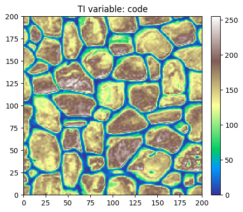
Training image (TI)
Read the TI and plot it. Source of the image: T. Zhang, P. Switzer, and A. Journel, Filter-based classification of training image patterns for spatial simulation, MATHEMATICAL GEOLOGY, 38(1):63-80, JAN 2006,*`doi:10.1007/s11004-005-9004-x <https://dx.doi.org/10.1007/s11004-005-9004-x>`__*.
[3]:
# Read file
data_dir = 'data'
filename = os.path.join(data_dir, 'tiContinuous.txt')
ti = gn.img.readImageTxt(filename)

# Color settings
cmap='terrain'
vmin, vmax = ti.vmin(), ti.vmax()

# Plot
plt.figure(figsize=(5,5))
gn.imgplot.drawImage2D(ti, cmap=cmap, vmin=vmin, vmax=vmax)
plt.title(f'TI variable: {ti.varname[0]}')
plt.show()
Simulation grid
Define the simulation grid (number of cells in each direction, cell unit, origin).
[4]:
nx, ny, nz = 200, 200, 1         # number of cells
sx, sy, sz = ti.sx, ti.sy, ti.sz # cell unit
ox, oy, oz = 0.0, 0.0, 0.0       # origin (corner of the "first" grid cell)
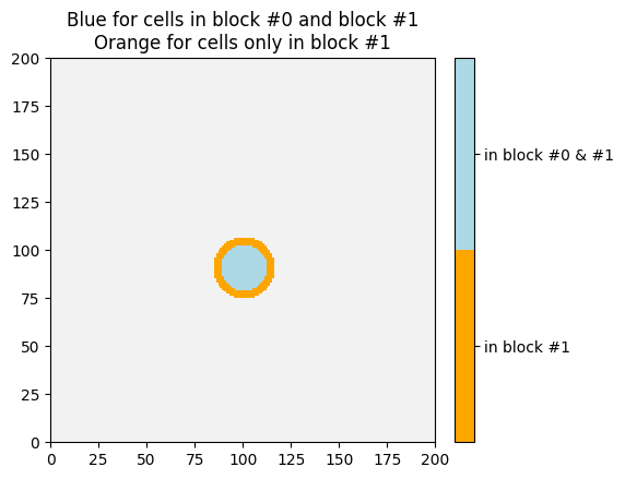
Define some block data
In this example, two block data are considered. The two block contain the simulation grid cells within a disk having the same center. Setting the first radius less than the second one, the first block is included in the second one.
[5]:
# disk center in the simulation grid
cx, cy = 100.5, 90.5
# radii
r0, r1 = 12., 16.

# coordinates of cell center
x = ox + sx*(0.5 + np.arange(nx))
y = oy + sy*(0.5 + np.arange(ny))
yy, xx = np.meshgrid(y, x, indexing='ij')

# index along x and y axes of the cells that are within each block
block_ind0 = np.where((xx-cx)**2 + (yy-cy)**2 < r0**2)
block_ind1 = np.where((xx-cx)**2 + (yy-cy)**2 < r1**2)
nodeIndex0 = [(i, j, 0) for j, i in zip(*block_ind0)]
nodeIndex1 = [(i, j, 0) for j, i in zip(*block_ind1)]

n0 = len(nodeIndex0)
n1 = len(nodeIndex1)

# target mean value for each block
v0 = 200. # mean value for the small disk
vc =  10. # mean value for the crown (large disk excluding the small one)
v1 = 1.0/n1*(n0*v0 + (n1-n0)*vc)  # mean value for the large disk (weigthed mean of v0 and vc)

# tolerance for each block
tol0 = 0.
tol1 = 0.

# activation proportion min for each block
amin0 = 0.0
amin1 = 0.0

# activation proportion max for each block
amax0 = .95
amax1 = .95

# block data
bd = gn.blockdata.BlockData(
    blockDataUsage=1,
    nblock=2,
    nodeIndex=[nodeIndex0, nodeIndex1],
    value=[v0, v1],
    tolerance=[tol0, tol1],
    activatePropMin=[amin0, amin1],
    activatePropMax=[amax0, amax1])

# Define image for viewing the block
im_block = gn.img.Img(nx, ny, nz, sx, sy, sz, ox, oy, oz, nv=1, val=0.0)
im_block.val[0][0][block_ind0] = im_block.val[0][0][block_ind0] + 1
im_block.val[0][0][block_ind1] = im_block.val[0][0][block_ind1] + 2
np.putmask(im_block.val, im_block.val==0, np.nan)

# figure
plt.figure(figsize=(5,5))
gn.imgplot.drawImage2D(im_block, categ=True, categCol=['orange', 'lightblue'],
                       cticklabels=['in block #1','in block #0 & #1'])
plt.title('Blue for cells in block #0 and block #1\nOrange for cells only in block #1')
plt.show()
Input for deesse and simulation
[6]:
nreal = 15
deesse_input = gn.deesseinterface.DeesseInput(
    nx=nx, ny=ny, nz=nz,
    sx=sx, sy=sy, sz=sz,
    ox=ox, oy=oy, oz=oz,
    nv=1, varname='code',
    TI=ti,
    distanceType='continuous',
    nneighboringNode=24,
    distanceThreshold=0.02,
    maxScanFraction=0.25,
    blockData=bd,             # block data
    npostProcessingPathMax=1,
    seed=444,
    nrealization=nreal)

# Run deesse
t1 = time.time() # start time
deesse_output = gn.deesseinterface.deesseRun(deesse_input)
t2 = time.time() # end time
print(f'Elapsed time: {t2-t1:.2g} sec')
deesseRun: DeeSse running... [VERSION 3.2 / BUILD NUMBER 20230914 / OpenMP 19 thread(s)]
deesseRun: DeeSse run complete
deesseRun: warnings encountered (1 times in all):
#  1: WARNING 00115: reproducibility is not guaranteed when using multiple threads and block data conditioning
Elapsed time: 37 sec
[7]:
# Retrieve the realizations
sim = deesse_output['sim']

# Gather the nreal realizations into one image
all_sim = gn.img.gatherImages(sim) # all_sim is one image with nreal variables

# Do statistics over all the realizations: compute the pixel-wise mean and standard deviation
sim_mean = gn.img.imageContStat(all_sim, op='mean') # do statistics (pixel-wise mean)
sim_std = gn.img.imageContStat(all_sim, op='std')   # do statistics (pixel-wise standard deviation)
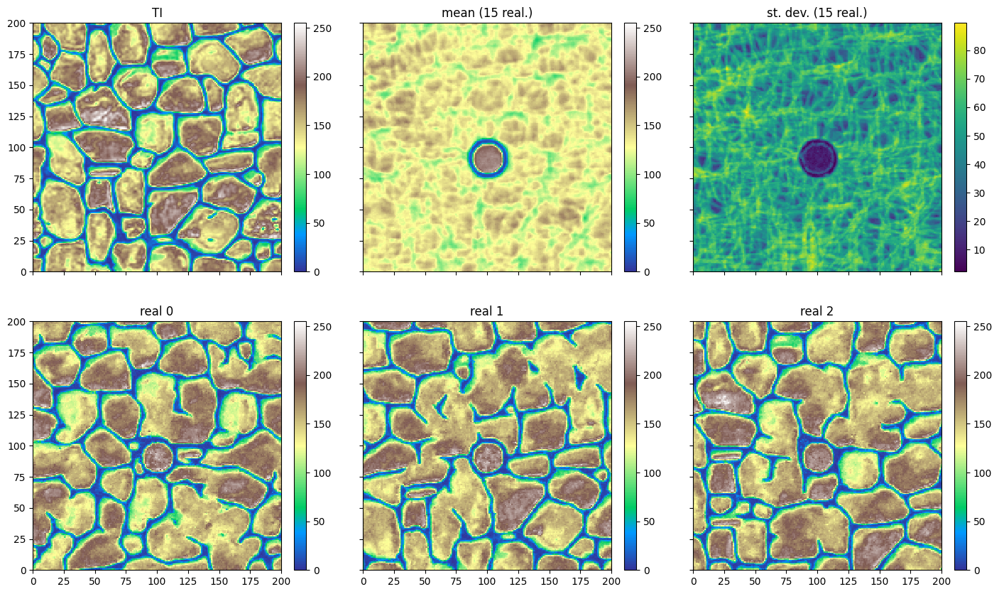
[8]:
# Figure
fig, ax = plt.subplots(2, 3, figsize=(17, 10), sharex=True, sharey=True)

# plot TI
plt.sca(ax[0, 0])
gn.imgplot.drawImage2D(ti, cmap=cmap, vmin=vmin, vmax=vmax, title='TI')

# plot mean of realizations
plt.sca(ax[0, 1])
gn.imgplot.drawImage2D(sim_mean, cmap=cmap, vmin=vmin, vmax=vmax, title=f'mean ({nreal} real.)')

# plot standard deviation of realizations
plt.sca(ax[0, 2])
gn.imgplot.drawImage2D(sim_std, title=f'st. dev. ({nreal} real.)')

# plot two realizations
for i in [0, 1, 2]:
    # plot real #i
    plt.sca(ax[1, i])
    gn.imgplot.drawImage2D(all_sim, iv=i, cmap=cmap, vmin=vmin, vmax=vmax, title=f'real {i}')

plt.show()
[9]:
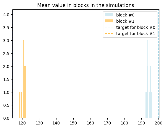
# Mean value in each block in the simulations
v_block = [
    np.mean(np.array([all_sim.val[:,k,j,i] for i, j, k in bd.nodeIndex[m]]).T, axis=1)
    for m in range(bd.nblock)]

# Histogram
plt.figure()
plt.hist(v_block[0], color='lightblue', alpha=.5, label='block #0')
plt.hist(v_block[1], color='orange',    alpha=.5, label='block #1')
plt.axvline(bd.value[0], color='lightblue', ls='dashed', label='target for block #0')
plt.axvline(bd.value[1], color='orange',    ls='dashed', label='target for block #1')
plt.title('Mean value in blocks in the simulations')
plt.legend()
plt.show()