GEONE - DEESSE - Simulation path and additional output maps

Main points addressed

• how to retrieve additional output maps from deesse (simulation path / error / TI grid node index / TI index)

• deesse simulations with different simulation path types

Import what is required

import numpy as np
import matplotlib.pyplot as plt
import time
import os

# import package 'geone'
import geone as gn

# Show version of python and version of geone
import sys
print(sys.version_info)
print('geone version: ' + gn.__version__)

sys.version_info(major=3, minor=13, micro=7, releaselevel='final', serial=0)
geone version: 1.3.0

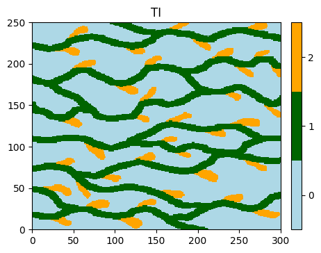
Training image (TI)

# Read file
data_dir = 'data'
filename = os.path.join(data_dir, 'ti.txt')
ti = gn.img.readImageTxt(filename)

# Values in the TI
ti.get_unique()

array([0., 1., 2.])

# Setting for categories / colors
categ_val = [0, 1, 2]
categ_col = ['lightblue', 'darkgreen', 'orange']

plt.figure(figsize=(5,5))
gn.imgplot.drawImage2D(ti, categ=True, categVal=categ_val, categCol=categ_col, title='TI')
plt.show()

Hard data (point set)

# Read the point set
data_dir = 'data'
filename = os.path.join(data_dir, 'hd.txt')
hd = gn.img.readPointSetTxt(filename)
hd

*** PointSet object ***
name = ''
npt = 7 # number of point(s)
nv = 4  # number of variable(s) (including coordinates)
varname = [np.str_('X'), np.str_('Y'), np.str_('Z'), np.str_('code')]
val: (4, 7)-array
*****

# For further plots:
# Get colors for hard data (according to variable of index 3 in the point set, and color settings)
hd_col = gn.imgplot.get_colors_from_values(hd.val[3], categ=True, categVal=categ_val, categCol=categ_col)
# # or equivalently:
# import matplotlib.colors
# hd_col=[matplotlib.colors.to_rgba(categ_col[int(v)]) for v in hd.val[3]] # colors (converted to 'rgba')
#                                                                          # of hard data points

Getting additional output from deesse (class geone.deesseinterface.DeesseInput)

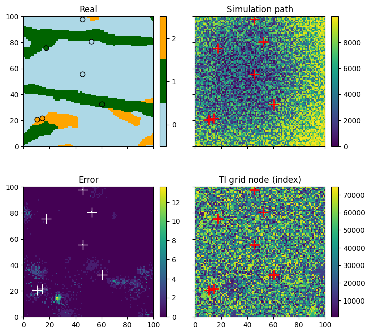
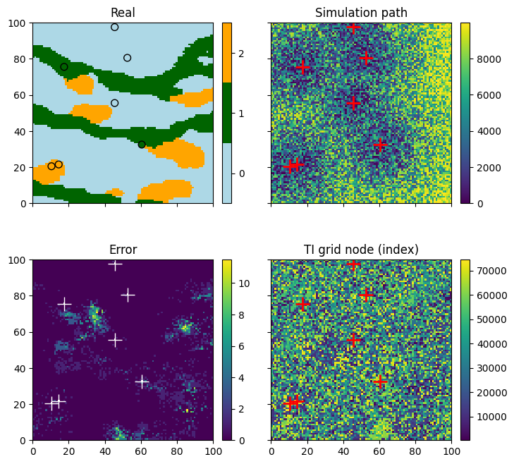
Additional information consisting of output maps (whose support is the simulation grid) can be retrieved in output when running deesse.

Simulation path map

It consists of an index attached to each simulation grid cell. The indexes give the order in which the cells are simulated.

Error map

It consists of the (relative) error attached to each simulation grid cell. The error is zero if the acceptation threshold has been reached, and positive otherwise. The error map highlights the regions where the simulation has been done without reaching the threshold and then where the reproduction of the structures might be poor.

TI grid node index map

It consists of an index attached to each simulation grid cell. The indexes give the index of the grid cell in the TI of the retained candidate during the simulation. The TI grid node index map can be useful for highlighting the regions in the simulation corresponding to verbatim copy of the TI.

TI index map

It consists of an index attached to each simulation grid cell. The indexes give the index of the TI that has been scanned during the simulation. Retrieving this map makes sense only if the number of TIs used is greater than one.

Remark In any of these maps, the value nan is set for cells that are not simulated, i.e conditioning cells or masked cells.

Filling the input structure for deesse and launch deesse

To get such maps in output, set corresponding flags (keyword arguments) to True:

• simulation path map: flag outputPathIndexFlag

• error map: flag outputErrorFlag

• TI grid node index map: flag outputTiGridNodeIndexFlag

• TI index map: flag outputTiIndexFlag

Note that, by default, these flags are set to False.

deesse_input = gn.deesseinterface.DeesseInput(
    nx=100, ny=100, nz=1,
    nv=1, varname='code',
    TI=ti,
    dataPointSet=hd,
    outputPathIndexFlag=True,       # get simulation path map in output (default: False)
    outputErrorFlag=True,           # get error map in output (default: False)
    outputTiGridNodeIndexFlag=True, # get TI grid node index map in output (default: False)
    distanceType='categorical',
    nneighboringNode=24,
    distanceThreshold=0.02,
    maxScanFraction=0.25,
    npostProcessingPathMax=1,
    seed=444,
    nrealization=1)

# Run deesse
t1 = time.time() # start time
deesse_output = gn.deesseinterface.deesseRun(deesse_input)
t2 = time.time() # end time
print(f'Elapsed time: {t2-t1:.2g} sec')

deesseRun: DeeSse running... [VERSION 3.2 / BUILD NUMBER 20230914 / OpenMP 19 thread(s)]
deesseRun: DeeSse run complete
Elapsed time: 0.91 sec

Retrieve the results (and display)

# Retrieve the realizations, the simulation path maps, the error maps and the TI grid node index maps (lists)
sim = deesse_output['sim']
path = deesse_output['path']
err = deesse_output['error']
tiGridNode = deesse_output['tiGridNode']

# Display
plt.subplots(2, 2, figsize=(8,8), sharex=True, sharey=True) # 2 x 2 sub-plots

plt.subplot(2, 2, 1)
gn.imgplot.drawImage2D(sim[0], categ=True, categVal=categ_val, categCol=categ_col, title='Real') # plot real
plt.scatter(hd.x(), hd.y(), marker='o', s=50, color=hd_col, edgecolors='black', lw=1) # add hard data points

plt.subplot(2, 2, 2)
gn.imgplot.drawImage2D(path[0], title='Simulation path') # plot simulation path
plt.plot(hd.x(), hd.y(), '+', markersize=15, c='r', markeredgewidth=2) # add hard data points

plt.subplot(2, 2, 3)
gn.imgplot.drawImage2D(err[0], title='Error') # plot error map
plt.plot(hd.x(), hd.y(), '+', markersize=15, c='white', markeredgewidth=1) # add hard data points

plt.subplot(2, 2, 4)
gn.imgplot.drawImage2D(tiGridNode[0], title='TI grid node (index)') # plot TI grid node index map
plt.plot(hd.x(), hd.y(), '+', markersize=15, c='r', markeredgewidth=2) # add hard data points

plt.show()

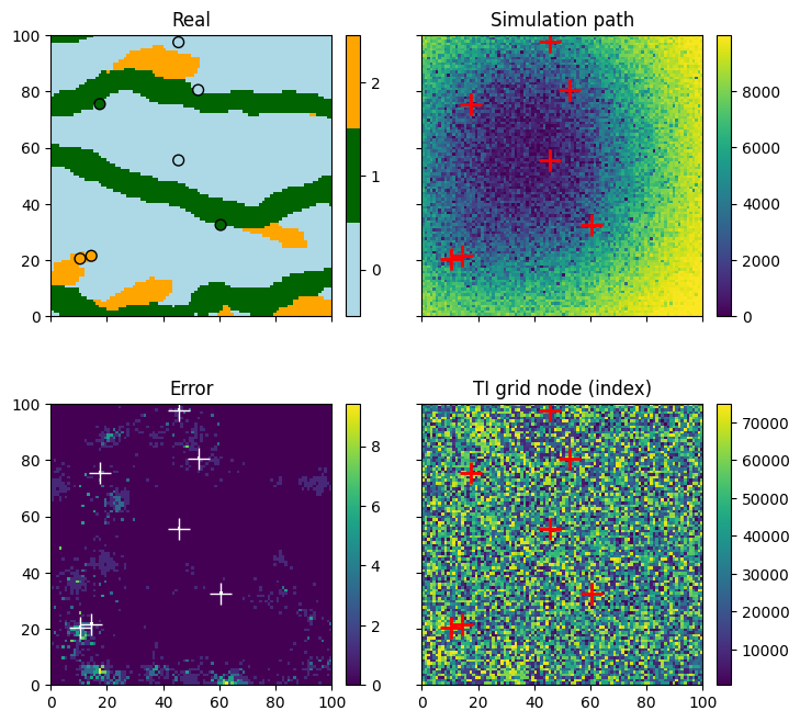
Specifying the simulation path type

Several types of simulation path are available. It is specified by the keyword argument simPathType (of the class geone.deesseinterface.DeesseInput), which is a character string:

• random: random path (default)

• random_hd_distance_pdf: random path set according to the distance to the ensemble of conditioning cells based on a probability distribution function (pdf): cells closer to a conditioning cell have a higher probability to be visited in the beginning of the path. It uses the keyword argument simPathStrength, a float in between 0 and 1: the closer to 1, more the path will be guided by the conditioning cells. (For unconditional simulation, one cell randomly chosen in the simulation grid will play the role of conditioning cell.)

• random_hd_distance_sort: random path set according to the distance to the ensemble of conditioning cells based on sort: the cells are sorted with respect to this distance combined with a random noise. It uses the keyword argument simPathStrength, a float in between 0 and 1: the closer to 1, more the path will be guided by the conditioning cells. (For unconditional simulation, one cell randomly chosen in the simulation grid will play the role of conditioning cell.)

• random_hd_distance_sum_pdf: random path set according to the sum of distances to the conditioning cells based on pdf. It uses the keyword argument simPathPower, a positive float to which the distances are raised before computing the sum, and the keyword argument simPathStrength, a float in between 0 and 1: the closer to 1, more the path will be guided by the conditioning cells. (For unconditional simulation, a random path is used.)

• random_hd_distance_sum_sort: random path set according to the sum of distances to the conditioning cells based on sort. It uses the keyword argument simPathPower, a positive float to which the distances are raised before computing the sum, and the keyword argument simPathStrength, a float in between 0 and 1: the closer to 1, more the path will be guided by the conditioning cells. (For unconditional simulation, a random path is used.)

• unilateral: unilateral path which uses the keyword argument simPathUnilateralOrder defining the order the axes (x, y, z[, v (variables)]) will be handled (see the doc by typing help(gn.deesseinterface.DeesseInput).

Some examples are given below.

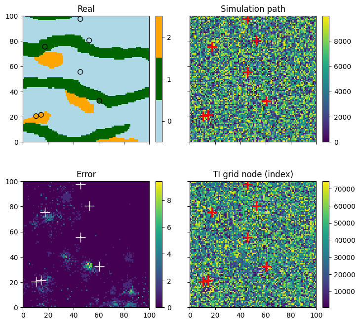
Random path according to the distance to hard data point set based on pdf

# path: 'random_hd_distance_pdf', strength: 0.8
deesse_input = gn.deesseinterface.DeesseInput(
    nx=100, ny=100, nz=1,
    nv=1, varname='code',
    TI=ti,
    dataPointSet=hd,
    outputPathIndexFlag=True,
    outputErrorFlag=True,
    outputTiGridNodeIndexFlag=True,
    simPathType='random_hd_distance_pdf',  # set simulation path type
    simPathStrength=0.8,                   #    set parameter for the path
    distanceType='categorical',
    nneighboringNode=24,
    distanceThreshold=0.02,
    maxScanFraction=0.25,
    npostProcessingPathMax=1,
    seed=444,
    nrealization=1)

# Run deesse
t1 = time.time() # start time
deesse_output = gn.deesseinterface.deesseRun(deesse_input)
t2 = time.time() # end time
print(f'Elapsed time: {t2-t1:.2g} sec')

deesseRun: DeeSse running... [VERSION 3.2 / BUILD NUMBER 20230914 / OpenMP 19 thread(s)]
deesseRun: DeeSse run complete
Elapsed time: 0.52 sec

# Retrieve the realizations, the simulation path maps, the error maps and the TI grid node index maps (lists)
sim = deesse_output['sim']
path = deesse_output['path']
err = deesse_output['error']
tiGridNode = deesse_output['tiGridNode']

# Display
plt.subplots(2, 2, figsize=(8,8), sharex=True, sharey=True) # 2 x 2 sub-plots

plt.subplot(2, 2, 1)
gn.imgplot.drawImage2D(sim[0], categ=True, categVal=categ_val, categCol=categ_col, title='Real') # plot real
plt.scatter(hd.x(), hd.y(), marker='o', s=50, color=hd_col, edgecolors='black', lw=1) # add hard data points

plt.subplot(2, 2, 2)
gn.imgplot.drawImage2D(path[0], title='Simulation path') # plot simulation path
plt.plot(hd.x(), hd.y(), '+', markersize=15, c='r', markeredgewidth=2) # add hard data points

plt.subplot(2, 2, 3)
gn.imgplot.drawImage2D(err[0], title='Error') # plot error map
plt.plot(hd.x(), hd.y(), '+', markersize=15, c='white', markeredgewidth=1) # add hard data points

plt.subplot(2, 2, 4)
gn.imgplot.drawImage2D(tiGridNode[0], title='TI grid node (index)') # plot TI grid node index map
plt.plot(hd.x(), hd.y(), '+', markersize=15, c='r', markeredgewidth=2) # add hard data points

plt.show()

Random path according to the distance to hard data point set based on sort

# path: 'random_hd_distance_sort', strength: 0.5
deesse_input = gn.deesseinterface.DeesseInput(
    nx=100, ny=100, nz=1,
    nv=1, varname='code',
    TI=ti,
    dataPointSet=hd,
    outputPathIndexFlag=True,
    outputErrorFlag=True,
    outputTiGridNodeIndexFlag=True,
    simPathType='random_hd_distance_sort',  # set simulation path type
    simPathStrength=0.5,                    #    set parameter for the path
    distanceType='categorical',
    nneighboringNode=24,
    distanceThreshold=0.02,
    maxScanFraction=0.25,
    npostProcessingPathMax=1,
    seed=444,
    nrealization=1)

# Run deesse
t1 = time.time() # start time
deesse_output = gn.deesseinterface.deesseRun(deesse_input)
t2 = time.time() # end time
print(f'Elapsed time: {t2-t1:.2g} sec')

deesseRun: DeeSse running... [VERSION 3.2 / BUILD NUMBER 20230914 / OpenMP 19 thread(s)]
deesseRun: DeeSse run complete
Elapsed time: 0.19 sec

# Retrieve the realizations, the simulation path maps, the error maps and the TI grid node index maps (lists)
sim = deesse_output['sim']
path = deesse_output['path']
err = deesse_output['error']
tiGridNode = deesse_output['tiGridNode']

# Display
plt.subplots(2, 2, figsize=(8,8), sharex=True, sharey=True) # 2 x 2 sub-plots

plt.subplot(2, 2, 1)
gn.imgplot.drawImage2D(sim[0], categ=True, categVal=categ_val, categCol=categ_col, title='Real') # plot real
plt.scatter(hd.x(), hd.y(), marker='o', s=50, color=hd_col, edgecolors='black', lw=1) # add hard data points

plt.subplot(2, 2, 2)
gn.imgplot.drawImage2D(path[0], title='Simulation path') # plot simulation path
plt.plot(hd.x(), hd.y(), '+', markersize=15, c='r', markeredgewidth=2) # add hard data points

plt.subplot(2, 2, 3)
gn.imgplot.drawImage2D(err[0], title='Error') # plot error map
plt.plot(hd.x(), hd.y(), '+', markersize=15, c='white', markeredgewidth=1) # add hard data points

plt.subplot(2, 2, 4)
gn.imgplot.drawImage2D(tiGridNode[0], title='TI grid node (index)') # plot TI grid node index map
plt.plot(hd.x(), hd.y(), '+', markersize=15, c='r', markeredgewidth=2) # add hard data points

plt.show()

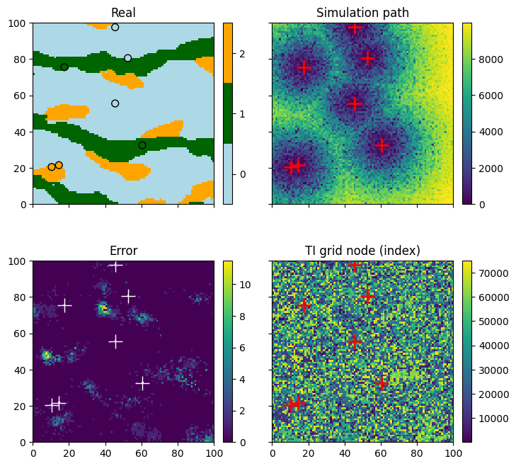
Random path according to the sum of distances to hard data points based on pdf

# path: 'random_hd_distance_sum_pdf', power: 1.0, strength: 0.8
deesse_input = gn.deesseinterface.DeesseInput(
    nx=100, ny=100, nz=1,
    nv=1, varname='code',
    TI=ti,
    dataPointSet=hd,
    outputPathIndexFlag=True,
    outputErrorFlag=True,
    outputTiGridNodeIndexFlag=True,
    simPathType='random_hd_distance_sum_pdf',  # set simulation path type
    simPathPower=1.0,                          #    set parameter for the path
    simPathStrength=0.8,                       #    set parameter for the path
    distanceType='categorical',
    nneighboringNode=24,
    distanceThreshold=0.02,
    maxScanFraction=0.25,
    npostProcessingPathMax=1,
    seed=444,
    nrealization=1)

# Run deesse
t1 = time.time() # start time
deesse_output = gn.deesseinterface.deesseRun(deesse_input)
t2 = time.time() # end time
print(f'Elapsed time: {t2-t1:.2g} sec')

deesseRun: DeeSse running... [VERSION 3.2 / BUILD NUMBER 20230914 / OpenMP 19 thread(s)]
deesseRun: DeeSse run complete
Elapsed time: 0.54 sec

# Retrieve the realizations, the simulation path maps, the error maps and the TI grid node index maps (lists)
sim = deesse_output['sim']
path = deesse_output['path']
err = deesse_output['error']
tiGridNode = deesse_output['tiGridNode']

# Display
plt.subplots(2, 2, figsize=(8,8), sharex=True, sharey=True) # 2 x 2 sub-plots

plt.subplot(2, 2, 1)
gn.imgplot.drawImage2D(sim[0], categ=True, categVal=categ_val, categCol=categ_col, title='Real') # plot real
plt.scatter(hd.x(), hd.y(), marker='o', s=50, color=hd_col, edgecolors='black', lw=1) # add hard data points

plt.subplot(2, 2, 2)
gn.imgplot.drawImage2D(path[0], title='Simulation path') # plot simulation path
plt.plot(hd.x(), hd.y(), '+', markersize=15, c='r', markeredgewidth=2) # add hard data points

plt.subplot(2, 2, 3)
gn.imgplot.drawImage2D(err[0], title='Error') # plot error map
plt.plot(hd.x(), hd.y(), '+', markersize=15, c='white', markeredgewidth=1) # add hard data points

plt.subplot(2, 2, 4)
gn.imgplot.drawImage2D(tiGridNode[0], title='TI grid node (index)') # plot TI grid node index map
plt.plot(hd.x(), hd.y(), '+', markersize=15, c='r', markeredgewidth=2) # add hard data points

plt.show()

Random path according to the sum of distances to hard data points based on sort

# path: 'random_hd_distance_sum_sort', power: 1.0, strength: 0.5
deesse_input = gn.deesseinterface.DeesseInput(
    nx=100, ny=100, nz=1,
    nv=1, varname='code',
    TI=ti,
    dataPointSet=hd,
    outputPathIndexFlag=True,
    outputErrorFlag=True,
    outputTiGridNodeIndexFlag=True,
    simPathType='random_hd_distance_sum_sort', # set simulation path type
    simPathPower=1.0,                          #    set parameter for the path
    simPathStrength=0.5,                       #    set parameter for the path
    distanceType='categorical',
    nneighboringNode=24,
    distanceThreshold=0.02,
    maxScanFraction=0.25,
    npostProcessingPathMax=1,
    seed=555,
    nrealization=1)

# Run deesse
t1 = time.time() # start time
deesse_output = gn.deesseinterface.deesseRun(deesse_input)
t2 = time.time() # end time
print(f'Elapsed time: {t2-t1:.2g} sec')

deesseRun: DeeSse running... [VERSION 3.2 / BUILD NUMBER 20230914 / OpenMP 19 thread(s)]
deesseRun: DeeSse run complete
Elapsed time: 0.15 sec

# Retrieve the realizations, the simulation path maps, the error maps and the TI grid node index maps (lists)
sim = deesse_output['sim']
path = deesse_output['path']
err = deesse_output['error']
tiGridNode = deesse_output['tiGridNode']

# Display
plt.subplots(2, 2, figsize=(8,8), sharex=True, sharey=True) # 2 x 2 sub-plots

plt.subplot(2, 2, 1)
gn.imgplot.drawImage2D(sim[0], categ=True, categVal=categ_val, categCol=categ_col, title='Real') # plot real
plt.scatter(hd.x(), hd.y(), marker='o', s=50, color=hd_col, edgecolors='black', lw=1) # add hard data points

plt.subplot(2, 2, 2)
gn.imgplot.drawImage2D(path[0], title='Simulation path') # plot simulation path
plt.plot(hd.x(), hd.y(), '+', markersize=15, c='r', markeredgewidth=2) # add hard data points

plt.subplot(2, 2, 3)
gn.imgplot.drawImage2D(err[0], title='Error') # plot error map
plt.plot(hd.x(), hd.y(), '+', markersize=15, c='white', markeredgewidth=1) # add hard data points

plt.subplot(2, 2, 4)
gn.imgplot.drawImage2D(tiGridNode[0], title='TI grid node (index)') # plot TI grid node index map
plt.plot(hd.x(), hd.y(), '+', markersize=15, c='r', markeredgewidth=2) # add hard data points

plt.show()