GEONE - Markov chains on finite sets
A Markov chain  on a finite set of states
  is a sequence of random variables such that the distribution a the next step
  depends only on the current step
  , which is known as the Markov property, or memorylessness.
Such random process is described by a transition kernel (or simply kernel), a  matrix
  with
with  and
and  . The coefficient
  is the probability to have the state
  at the next step given the state
  at the current step, i.e.
This notebook illustrates some tools available in GEONE to deal with the simulation of Markov chains on finite sets.
Import what is required
[1]:
import numpy as np
import matplotlib.pyplot as plt

from matplotlib.gridspec import GridSpec

# import package 'geone'
import geone as gn
[2]:
# Show version of python and version of geone
import sys
print(sys.version_info)
print('geone version: ' + gn.__version__)
sys.version_info(major=3, minor=13, micro=7, releaselevel='final', serial=0)
geone version: 1.3.1
Markov chains on finite sets - basic background theory
With the notations above, and denoting  the probability mass function (pmf) over
  at step of the Markov chain,
  , i.e.
 ,
,
we have

where  is the transition kernel of the chain.
Convergence of Markov chains
If the graph associated to the transition kernel is connected, then it exists a unique invariant pmf  and, for any starting
  , the distribution of
  conveges towards . The chain
  is said stationary.
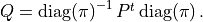
Let  be the reverse transition kernel, i.e.
  is the probability to have the state at the previous step given the state at the current step. We have

If denotes the invariant pmf of the chain (assuming it exists), i.e.  , and if
  , then we have
  and
and 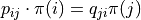 , i.e.
Symmetric transition kernel
If is symmetric, then  is invariant, because the columns of are the lines of and they sum to one. It follows that
  .
.
Covariance of Markov chains
Let  the indicator variable for the state at step (i.e. with value
  if
if  and
and  otherwise). Assuming the chain is stationary, i.e. converging towards
  , we have for large :

and for  :
:

As
$
$
we have
![\operatorname{cov}\left(\mathbf{1}_{X_k=i}, \mathbf{1}_{X_{k+l}=j}\right) \approx \pi(i) \left[\left(P^l\right)_{ij}-\pi(j)\right].](../_images/math/39fac3f1d71a25e6c6a66999d5b13ff8ffd9c742.png)
Pre-defined kernels
The module geone.markovChain provides functions to define specific kernels.
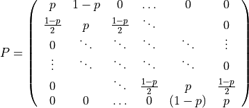
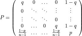
Kernel - function geone.markovChain.mc_kernel1
This function sets (returns) the symmetric kernel
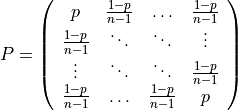
where  . The associated graph is connected and then any chain is stationary.
According to this kernel, from one step to the next one:
the state remains unchanged with probability
 ,
,the state changes to any other state with probability
 .
.
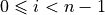
As is symmetric, the invariant distribution is 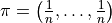 .
.
Kernel - function geone.markovChain.mc_kernel2
This function sets (returns) the kernel
where . The associated graph is connected and then any chain is stationary.
According to this kernel, from one step to the next one:
the state remains unchanged with probability
,the state
,  , changes to the state at right (
 ) or at left (
 ) with probability
  ,
,the state
(resp.  ) changes to the state (reps.
  ) with probability
  .
.
The invariant distribution is 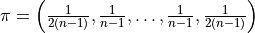 .
.
Kernel - function geone.markovChain.mc_kernel3
This function sets (returns) the kernel
where and  are independent. The associated graph is connex and then any chain is stationary.
According to this kernel, from one step to the next one:
the state remains unchanged with probability
,the state (
) changes to the state at right () with probability  (identifying “state
  ” with state ), and to the state at left () with probabibility
  , (identifying “state
  ” with state ).
As the sum of each column in is equal to one, the invariant distribution is . Note that if  , the kernel is symmetric.
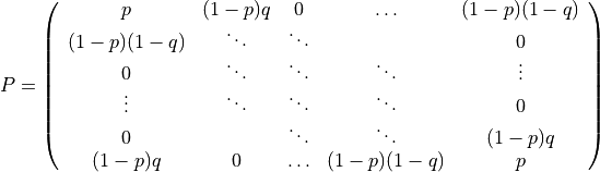
Kernel - function geone.markovChain.mc_kernel4
This function sets (returns) the kernel
where and  are independent. The associated graph is connex and then any chain is stationary.
According to this kernel, from one step to the next one:
the state
 remains unchanged with probability
  and change to the state with probability
  ,
,the state
 remains unchanged with probability and change to any other state with probability .
The invariant distribution is 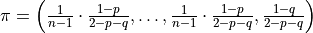 . Note that if
  , the kernel is symmetric.
Simulation of Markov chains
Settings
Define number of categories (states), their values and the transition kernel.
[3]:
# Y: stationary stochastic process given by a markov chain
# --------------------------------------------------------

# --------------------------------------------------------------
# Categories
# ----------
# Number of categories (states)
ncat = 4

# Category values
categVal = np.array([1, 2, 3, 4])

# Category colors (for further plot)
categCol = ['lightblue', 'darkgreen', 'orange', 'brown']

# Transition kernel
# -----------------
p = 0.95
kernel = gn.markovChain.mc_kernel1(ncat, p)  # kernel #1
# --------------------------------------------------------------
[4]:
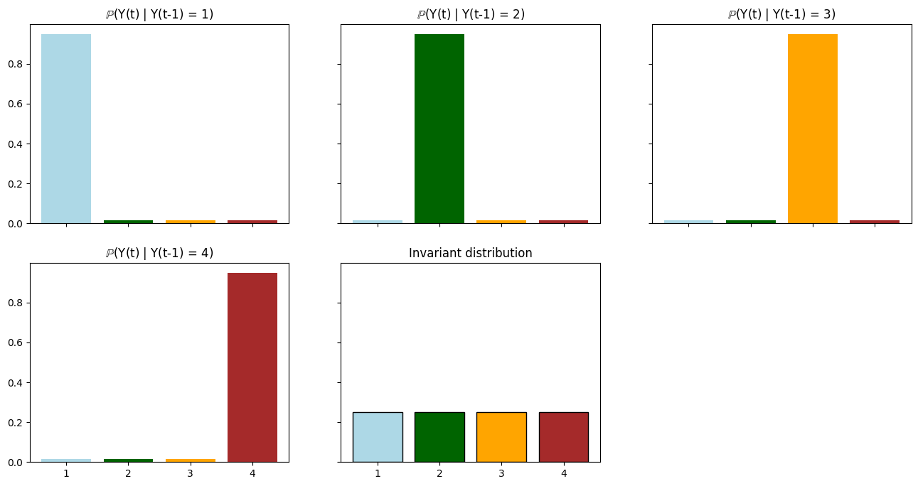
# Invariant distribution
pinv = gn.markovChain.compute_mc_pinv(kernel)

# Plot transition probabilities and invariant distribution
# --------------------------------------------------------
nf = ncat + 1
nr = int(np.sqrt(nf))
nc = nf // nr + 1*(nf%nr > 0)
hmin = 0.0
hmax = 1.05*max(kernel.max(), pinv.max())

plt.subplots(nr, nc, sharex=True, sharey=True, figsize=(16,8))

for i in range(ncat):
    plt.subplot(nr, nc, i+1)
    plt.bar(np.arange(ncat), kernel[i], color=categCol, tick_label=categVal)
    plt.ylim((hmin, hmax))
    plt.title(r'$\mathbb{P}$' + f'(Y(t) | Y(t-1) = {categVal[i]})')

plt.subplot(nr, nc, ncat+1)
plt.bar(np.arange(ncat), pinv, color=categCol, edgecolor='black', tick_label=categVal)
plt.ylim((hmin, hmax))
plt.title(f'Invariant distribution')

for i in range(ncat+2, nr*nc+1):
    plt.subplot(nr, nc, i)
    plt.axis('off')

plt.show()
Generate unconditional Markov chains
[5]:
# Unconditional markov chain
# --------------------------
# Length of the chain
ylength = 50000
# Simulation
np.random.seed(123)
y = gn.markovChain.simulate_mc(kernel, ylength, categVal=categVal, nreal=1)
# -> y is an array of shape (nreal, length)
# Compute empirical invariant distribution
pinv_emp = np.array([np.mean(y==categVal[i]) for i in range(ncat)])
# Compute empirical covariance function
nlag = 40
cov_y_emp = np.zeros((nlag, ncat, ncat))
for i in range(ncat):
for j in range(ncat):
cov_y_emp[:, i, j] = np.array(
[np.cov(y[0,m:]==categVal[j], y[0,:y.shape[1]-m]==categVal[i])[0,1] for m in range(nlag)])
# Theoretical covariances
cov_y = gn.markovChain.compute_mc_cov(kernel, nsteps=nlag)
print("Kernel:\n", kernel)
print("Invariant distribution, empirical (pinv_emp):", pinv_emp)
print("Invariant distribution, theoretical (pinv) :", pinv)
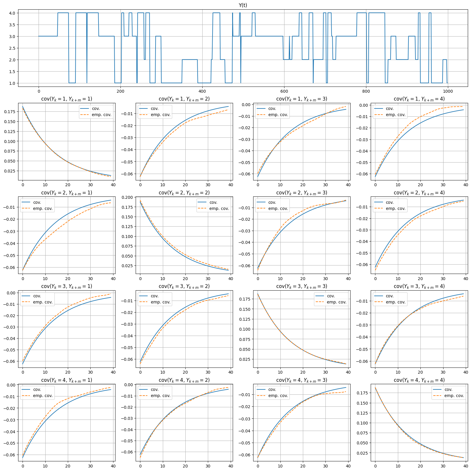
# Plot Y simulation and covariances
# ---------------------------------
fig = plt.figure(figsize=(16, 16), constrained_layout=True)
gs = GridSpec(ncat+1, ncat, figure=fig)
ax = fig.add_subplot(gs[0, :])
plt.sca(ax)
plt.plot(y[0,:min(ylength, 1000)])
plt.grid()
plt.title('Y(t)')
for i in range(ncat):
for j in range(ncat):
ax = fig.add_subplot(gs[1+i, j])
plt.sca(ax)
ax.plot(cov_y[:,i,j], label='cov.')
plt.plot(cov_y_emp[:,i,j], ls='dashed', label='emp. cov.')
plt.legend()
plt.grid()
plt.title('cov($Y_{}={}$, $Y_{}={}$)'.format('{k}', categVal[i], '{k+m}', categVal[j]))
plt.show()
Kernel:
 [[0.95       0.01666667 0.01666667 0.01666667]
 [0.01666667 0.95       0.01666667 0.01666667]
 [0.01666667 0.01666667 0.95       0.01666667]
 [0.01666667 0.01666667 0.01666667 0.95      ]]
Invariant distribution, empirical (pinv_emp): [0.2412  0.25938 0.24802 0.2514 ]
Invariant distribution, theoretical (pinv)  : [0.25 0.25 0.25 0.25]
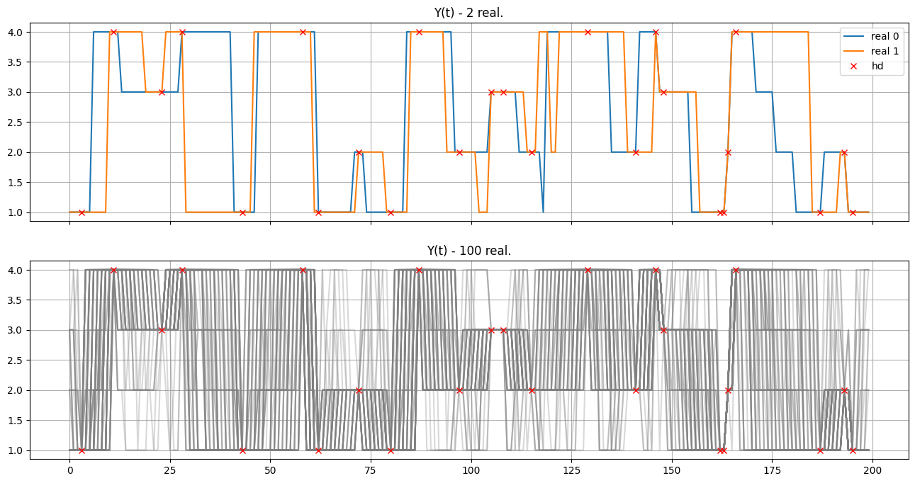
[6]:
# Conditional markov chain
# ------------------------
# Length of the chain
ylength = 200

# Conditioning points
nhd = 25
np.random.seed(85938)
yind = np.random.choice(ylength, size=nhd, replace=False)
yval = np.random.choice(categVal, size=nhd, replace=True)

# Simulation
np.random.seed(123)
nreal=100
y = gn.markovChain.simulate_mc(kernel, ylength, categVal=categVal, data_ind=yind, data_val=yval, nreal=nreal)

# Plot 2 real. and ensemble of real.
# ----------------------------------
plt.subplots(2,1, sharex=True, figsize=(16, 8))
plt.subplot(2,1,1)

plt.plot(y[0, :min(ylength, 1000)], label=f'real 0')
plt.plot(y[1, :min(ylength, 1000)], label=f'real 1')
plt.plot(yind, yval, 'rx', label='hd')
plt.grid()
plt.legend()
plt.title('Y(t) - 2 real.')

plt.subplot(2,1,2)
for i in range(nreal):
    plt.plot(y[i, :min(ylength, 1000)], c='gray', alpha=.3)

plt.plot(yind, yval, 'rx')
plt.grid()
plt.title(f'Y(t) - {nreal} real.')
plt.show()