GEONE - GEOSCLASSIC - Two-point statistics analysis of images

Two-point statistics analysis of image

image of covariance, variogram, correlogram (correlation)
geobody (connected component) image
image of connectivity functions
Gamma and Euler number connectivity indicator (curve)

Remark: examples in 2D are proposed here.

Import what is required

[1]:

import numpy as np
import matplotlib.pyplot as plt

# import package 'geone'
import geone as gn

[2]:

# Show version of python and version of geone
import sys
print(sys.version_info)
print('geone version: ' + gn.__version__)

sys.version_info(major=3, minor=13, micro=7, releaselevel='final', serial=0)
geone version: 1.3.1

Remark

The matplotlib figures can be visualized in interactive mode:

%matplotlib notebook: enable interactive mode
%matplotlib inline: disable interactive mode

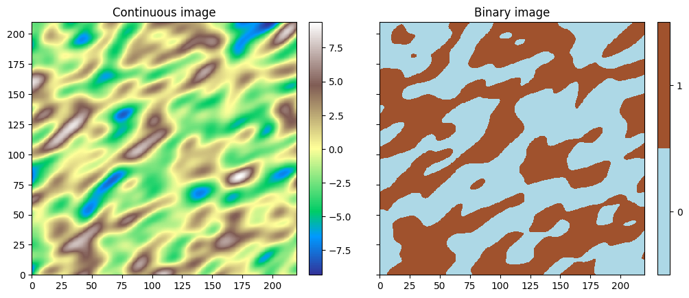
Generate a continuous image and a binary image (2D)

To illustrate the image analysis tools, an initial continuous image (variable $v$ ) is generated (Gaussian Random Field, see jupyter notebook ex_grf_2d), and a binary image is obtained by considering the indicator variable $I(x)=1 \iff v(x)>0$ , i.e. setting the value $1$ where the continuous variable is greater than $0$ and the value $0$ elsewhere.

[3]:

cov_model = gn.covModel.CovModel2D(elem=[
    ('gaussian', {'w':9, 'r':[30, 15]}),   # elementary contribution (different ranges: anisotropic)
    #('nugget', {'w':0.5})                   # elementary contribution
    ], alpha=-30.0, name='ref model (anisotropic)')

# Simulation grid (domain)
nx, ny = 440, 420  # number of cells
dx, dy = 0.5, 0.5  # cell unit
ox, oy = 0.0, 0.0  # origin

# Simulation
np.random.seed(222)
v = gn.grf.grf2D(cov_model, (nx, ny), (dx, dy), (ox, oy), nreal=1)
    # 3d-array of shape 1 x ny x nx

# Define image containing the simulation
im_cont = gn.img.Img(nx, ny, 1, dx, dy, 1., ox, oy, 0., nv=1, val=v) # fill image (Img class from geone.img)

# Define the binary image
im_bin = gn.img.Img(nx, ny, 1, dx, dy, 1., ox, oy, 0., nv=1, val=(v>0))

# Display images
col_bin = ['lightblue', 'sienna']
plt.subplots(1,2,figsize=(12,8), sharey=True)

plt.subplot(1,2,1)
gn.imgplot.drawImage2D(im_cont, cmap='terrain', title='Continuous image')

plt.subplot(1,2,2)
gn.imgplot.drawImage2D(im_bin, categ=True, categVal=[0,1], categCol=col_bin, title='Binary image')

plt.show()

../_images/notebooks_ex_geosclassic_image_analysis_5_0.png

Basic two-point statistics

Function `geone.geosclassicinterface.imgTwoPointStatisticsImage`

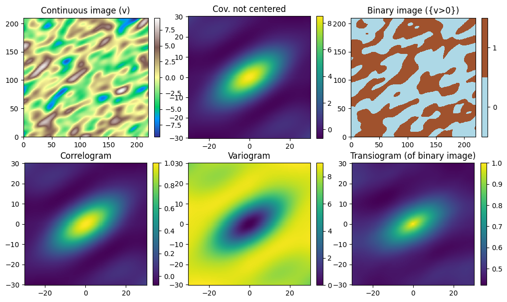
The function geone.geosclassicinterface.imgTwoPointStatisticsImage allows to compute different types of two-point statistics for a variable $v$ in an input image and produces an output image of the chosen statistics for lag $h$ covering a grid, The following types of two-point statistics are available and passed to the function through the keyword argument stat_type (string):

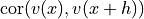$\operatorname{cor}(v(x), v(x+h))$ : Pearson correlation, stat_type='correlogram'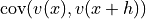
$\operatorname{cov}(v(x), v(x+h))$ : covariance, stat_type='covariance' (default)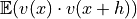
$\mathbb{E}(v(x)\cdot v(x+h))$ : covariance not centered, stat_type='covariance_not_centered'
$\mathbb{P}(v(x+h)>0 \vert v(x)>0)$ : transiogram, stat_type='transiogram'
$1/2\cdot\mathbb{E}\left((v(x)-v(x+h)^2\right)$ : variogram, stat_type='variogram'

Note that a transiogram is computed for the indicator variable $I(x)$ defined as $I(x)=1 \iff v(x)>0$ (the binary image).

The minimal lag, maximal lag and the lag step in each direction are expressed in number of cells (in the input image minimal) and passed to the function with the keyword arguments hx_min, hx_max, hx_step (resp. hy_min, hy_max, hy_step and hz_min, hz_max, hz_step) for the $x$ -axis direction (resp. for the $y$ and $z$ -axis directions). For example, hx_min=-10, hx_max=10, hx_step=2 implies that lags in $x$ -axis direction of -10, -8, -6, -4, -2, 0, 2, 4, 6, 8, 10 cells (in input image) will be considered.

By default, the minimal and maximal lags are set to $\pm$ one half of the number of cells in the corresponding direction, and the lag step is set to 1.

The variable $v$ (in input image) of index var_index (keyword argument, default: 0) is considered.

This function launches a C program running in parallel (based on OpenMP). The number of threads used can be specified by the optional parameter (keyword argument) nthreads. Specifying for this parameter a number -n, negative or zero, means that the total number of cpus of the system (retrieved by os.cpu_count()) except n (but at least one) will be used. By default: nthreads=-1.

[4]:

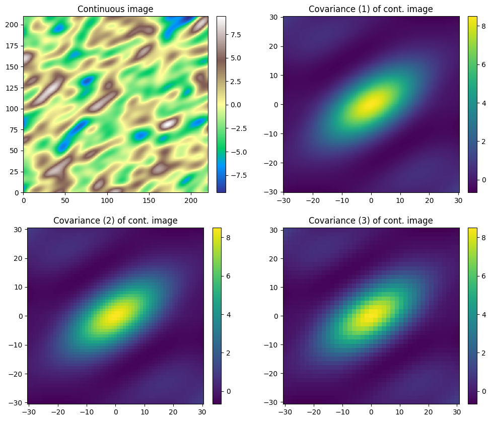
# For the continuous image:
# compute covariance map with different resolutions
im_cont_cov_1 = gn.geosclassicinterface.imgTwoPointStatisticsImage(im_cont,
                                                                   hx_min=-60, hx_max=60, #hx_step=1,
                                                                   hy_min=-60, hy_max=60, #hy_step=1,
                                                                   #hz_min=0,   hz_max=0,  hz_step=1
                                                                   #nthreads=-1
                                                                  )
im_cont_cov_2 = gn.geosclassicinterface.imgTwoPointStatisticsImage(im_cont,
                                                                   hx_min=-60, hx_max=60, hx_step=2,
                                                                   hy_min=-60, hy_max=60, hy_step=2)
im_cont_cov_3 = gn.geosclassicinterface.imgTwoPointStatisticsImage(im_cont,
                                                                   hx_min=-60, hx_max=60, hx_step=3,
                                                                   hy_min=-60, hy_max=60, hy_step=3)

# Display images
plt.subplots(2,2,figsize=(12,10))

plt.subplot(2,2,1)
gn.imgplot.drawImage2D(im_cont, cmap='terrain', title='Continuous image')

plt.subplot(2,2,2)
gn.imgplot.drawImage2D(im_cont_cov_1, cmap='viridis', title='Covariance (1) of cont. image')

plt.subplot(2,2,3)
gn.imgplot.drawImage2D(im_cont_cov_2, cmap='viridis', title='Covariance (2) of cont. image')

plt.subplot(2,2,4)
gn.imgplot.drawImage2D(im_cont_cov_3, cmap='viridis', title='Covariance (3) of cont. image')

plt.show()

../_images/notebooks_ex_geosclassic_image_analysis_7_0.png

[5]:

print('covariance map 1: {} x {}, cell size = {} x {}'.format(im_cont_cov_1.nx, im_cont_cov_1.ny,
                                                              im_cont_cov_1.sx, im_cont_cov_1.sy))
print('covariance map 2: {} x {}, cell size = {} x {}'.format(im_cont_cov_2.nx, im_cont_cov_2.ny,
                                                              im_cont_cov_2.sx, im_cont_cov_2.sy))
print('covariance map 3: {} x {}, cell size = {} x {}'.format(im_cont_cov_3.nx, im_cont_cov_3.ny,
                                                              im_cont_cov_3.sx, im_cont_cov_3.sy))

covariance map 1: 121 x 121, cell size = 0.5 x 0.5
covariance map 2: 61 x 61, cell size = 1.0 x 1.0
covariance map 3: 41 x 41, cell size = 1.5 x 1.5

[6]:

# Compute other two-point statistics
im_cont_cov_nc = gn.geosclassicinterface.imgTwoPointStatisticsImage(im_cont,
                    hx_min=-60, hx_max=60, hy_min=-60, hy_max=60, stat_type='covariance_not_centered')
im_cont_cor = gn.geosclassicinterface.imgTwoPointStatisticsImage(im_cont,
                    hx_min=-60, hx_max=60, hy_min=-60, hy_max=60, stat_type='correlogram')
im_cont_vario = gn.geosclassicinterface.imgTwoPointStatisticsImage(im_cont,
                    hx_min=-60, hx_max=60, hy_min=-60, hy_max=60, stat_type='variogram')
im_bin_transio = gn.geosclassicinterface.imgTwoPointStatisticsImage(im_bin, # (or im_cont)
                    hx_min=-60, hx_max=60, hy_min=-60, hy_max=60, stat_type='transiogram')

# Display images
plt.subplots(2,3,figsize=(12,7))

plt.subplot(2,3,1)
gn.imgplot.drawImage2D(im_cont, cmap='terrain', title='Continuous image (v)')

plt.subplot(2,3,2)
gn.imgplot.drawImage2D(im_cont_cov_nc, cmap='viridis', title='Cov. not centered')

plt.subplot(2,3,3)
gn.imgplot.drawImage2D(im_bin, categ=True, categVal=[0,1], categCol=col_bin, title='Binary image ({v>0})')

plt.subplot(2,3,4)
gn.imgplot.drawImage2D(im_cont_cor, cmap='viridis', title='Correlogram')

plt.subplot(2,3,5)
gn.imgplot.drawImage2D(im_cont_vario, cmap='viridis', title='Variogram')

plt.subplot(2,3,6)
gn.imgplot.drawImage2D(im_bin_transio, cmap='viridis', title='Transiogram (of binary image)')

plt.show()

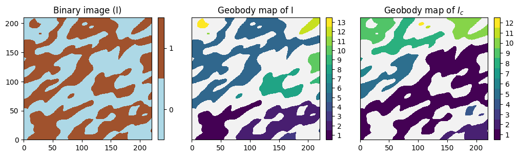
../_images/notebooks_ex_geosclassic_image_analysis_9_0.png

Connectivity: geobody image

Function `geone.geosclassicinterface.imgGeobodyImage`

The function geone.geosclassicinterface.imgGeobodyImage computes the geobody image (map) of a binary image. The output image has the same grid geometry as the input image and one variable consisting of the geobody label in the set $\{I=1\}$ from the input image (and value $0$ for cell in the set $\{I=0\}$ ).

The definition of adjacent cells depends on the keyword argument connect_type (string):

connect_type='connect_face' (default): two grid cells are adjacent if they have a common face
connect_type='connect_face_edge': two grid cells are adjacent if they have a common face or a common edge
connect_type='connect_face_edge_corner': two grid cells are adjacent if they have a common face or a common edge or a common corner

A continuous image (variable $v$ ) can be given in input, it is then transformed into a binary image (variable $I$ ) according to the keyword argument bound_inf (default: $0$ ), bound_sup (default: “ $+\infty$ ”)(floats), and bound_inf_excluded, bound_sup_excluded (booleans):

$I(x) = 1 \iff$ bound_inf $< v(x) <$ bound_sup if bound_inf_excluded is True and bound_sup_excluded is True (default)
$I(x) = 1 \iff$ bound_inf $< v(x) \leqslant$ bound_sup if bound_inf_excluded is True and bound_sup_excluded is False
$I(x) = 1 \iff$ bound_inf $\leqslant v(x) <$ bound_sup if bound_inf_excluded is False and bound_sup_excluded is True
$I(x) = 1 \iff$ bound_inf $\leqslant v(x) \leqslant$ bound_sup if bound_inf_excluded is False and bound_sup_excluded is False

Moreover, the keyword argument complementary_set (boolean) indicates that the variable $I_c(x) = 1-I(x)$ is used instead $I$ if True, i.e. the complementary binary image is considered. Default: False (variable $I$ is considered).

The variable $v$ (in input image) of index var_index (keyword argument, default: 0) is considered.

This function launches a C program (running in serial).

The algorithm used is described in Hoshen and Kopelman (1976) Physical Review B, 14(8):3438.

[7]:

# Compute geobody map of the binary image
im_bin_geo = gn.geosclassicinterface.imgGeobodyImage(im_bin)
im_bin_c_geo = gn.geosclassicinterface.imgGeobodyImage(im_bin, complementary_set=True)

# Display images
plt.subplots(1,3,figsize=(12,8))

plt.subplot(1,3,1)
gn.imgplot.drawImage2D(im_bin, categ=True, categVal=[0,1], categCol=col_bin, title='Binary image (I)')

plt.subplot(1,3,2)
gn.imgplot.drawImage2D(im_bin_geo, categ=True, categVal=np.arange(1,im_bin_geo.val.max()+1),
                       yticks=[], title='Geobody map of I')
# value 0 not included in categVal so that it is not displayed

plt.subplot(1,3,3)
gn.imgplot.drawImage2D(im_bin_c_geo, categ=True, categVal=np.arange(1,im_bin_c_geo.val.max()+1),
                       yticks=[], title='Geobody map of $I_c$')

plt.show()

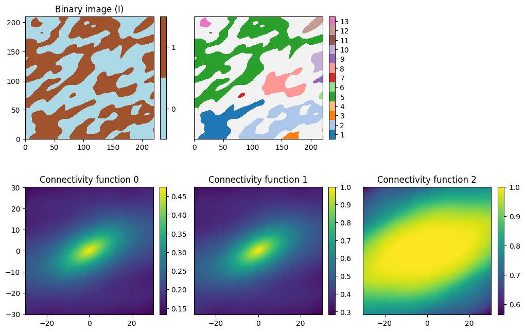
../_images/notebooks_ex_geosclassic_image_analysis_11_0.png

Connectivity analysis: ‘’connectogram’’

Function `geone.geosclassicinterface.imgTwoPointStatisticsImage`

The function geone.geosclassicinterface.imgTwoPointStatisticsImage also allows to compute probability of connection between two pairs of points as function as the lag between their locations.

The input image must be the geobody image of the underlying indicator variable I considered (computed using the function geone.geosclassicinterface.imgGeobodyImage). Let $C$ be the variable given the geobody label (equals to 0 if in no geobody), and let write $x\leftrightarrow y$ if the cells located at $x$ and $y$ are connected, i.e. in the same geobody. Three connectivity function can be computed and specified by the keyword argument stat_type (string):

$\mathbb{P}(x\leftrightarrow x+h) = \mathbb{P}(C(x) = C(x+h) > 0)$ : stat_type='connectivity_func0'
$\mathbb{P}(x\leftrightarrow x+h|I(x)=1) = \mathbb{P}(C(x) = C(x+h)|C(x) > 0)$ : stat_type='connectivity_func1'
$\mathbb{P}(x\leftrightarrow x+h|I(x)=I(x+h)=1) = \mathbb{P}(C(x) = C(x+h) > 0|C(x), C(x+h) > 0)$ : stat_type='connectivity_func2'

In particular, we have the following relation:

$\mathbb{P}(x \leftrightarrow x+h) = \mathbb{P}(x \leftrightarrow x+h | I(x)=I(x+h)=1)\cdot\mathbb{E}(I(x)\cdot I(x+h))$

i.e “connectivity_func0 = connectivity_func2 * covariance_not_centered”.

See reference: Renard P, Allard D (2013), Connectivity metrics for subsurface flow and transport. Adv Water Resour 51:168–196,doi:10.1016/j.advwatres.2011.12.001.

The minimal lag, maximal lag and the lag step in each direction are expressed in number of cells and specified as explained above. The variable $v$ (in input image) of index var_index (keyword argument, default: 0) is considered. This function launches a C program running in parallel, the number of threads used (keyword argument nthreads, see above) can be specified.

[8]:

# Compute connectivity functions for the binary image im_bin
im_bin_geo = gn.geosclassicinterface.imgGeobodyImage(im_bin) # geobody image (already computed)

im_bin_connect0 = gn.geosclassicinterface.imgTwoPointStatisticsImage(im_bin_geo,
                    hx_min=-60, hx_max=60, hy_min=-60, hy_max=60, stat_type='connectivity_func0')
im_bin_connect1 = gn.geosclassicinterface.imgTwoPointStatisticsImage(im_bin_geo,
                    hx_min=-60, hx_max=60, hy_min=-60, hy_max=60, stat_type='connectivity_func1')
im_bin_connect2 = gn.geosclassicinterface.imgTwoPointStatisticsImage(im_bin_geo,
                    hx_min=-60, hx_max=60, hy_min=-60, hy_max=60, stat_type='connectivity_func2')

# Display images
plt.subplots(2,3,figsize=(12,8))

plt.subplot(2,3,1)
gn.imgplot.drawImage2D(im_bin, categ=True, categVal=[0,1], categCol=col_bin, title='Binary image (I)')

plt.subplot(2,3,2)
gn.imgplot.drawGeobodyMap2D(im_bin_geo)
plt.yticks([])
# gn.imgplot.drawImage2D(im_bin_geo, categ=True, categVal=np.arange(1,im_bin_geo.val.max()+1),
#                        yticks=[], title='Geobody map of I')

plt.subplot(2,3,3)
plt.axis('off')

plt.subplot(2,3,4)
gn.imgplot.drawImage2D(im_bin_connect0, cmap='viridis', title='Connectivity function 0')

plt.subplot(2,3,5)
gn.imgplot.drawImage2D(im_bin_connect1, cmap='viridis', yticks=[], title='Connectivity function 1')

plt.subplot(2,3,6)
gn.imgplot.drawImage2D(im_bin_connect2, cmap='viridis', yticks=[], title='Connectivity function 2')

plt.show()

../_images/notebooks_ex_geosclassic_image_analysis_13_0.png

Connectivity analysis: Gamma value and Euler number

The functions geone.geosclassicinterface.imgConnectivityGammaValue and geone.geosclassicinterface.imgConnectivityEulerNumber computes the Gamma value and the Euler number for a binary image (or for the indicator variable 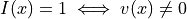$I(x)= 1 \iff v(x) \neq 0$ of a continuous image with variable $v$ ).

Gamma value

The Gamma value is a global measure of connectivity and is defined as

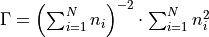
$\Gamma = \left(\sum_{i=1}^N n_i\right)^{-2} \cdot \sum_{i=1}^N n_i^2$

where $N$ is the number of connected components (geobodies) of the set $\{I=1\}$ and $n(i)$ the number of cells in the $i$ -th geobody (geobody of label $i$ ). Hence, $\Gamma$ is the probability that two cells (possibly the same ones) taken randomly in the set $\{I=1\}$ are connected.

Euler number

The Euler number $E$ gives the number of connected components (geobodies) + the number of ‘’holes’’ - the number of ‘’handles’’ in the set $\{I=1\}$ , and can be computed by the formula

$E = \sum_{i=1,...,N} (e0_i - e1_i + e2_i - e3_i)$

where $N$ the number of connected component (geobodies) in the set {I=1} and

$e0_i$ is the number of vertices (element of dimension 0) in the $i$ -th geobody
$e1_i$ is the number of edges (element of dimension 1) in the $i$ -th geobody
$e2_i$ is the number of faces (element of dimension 2) in the $i$ -th geobody
$e3_i$ is the number of volumes (cells, element of dimension 3) in the $i$ -th geobody

where vertices, edges, faces, and volumes of any grid cell (3D parallelepiped element) are considered.

See reference: Renard P, Allard D (2013), Connectivity metrics for subsurface flow and transport. Adv Water Resour 51:168–196,doi:10.1016/j.advwatres.2011.12.001.

Function `geone.geosclassicinterface.imgConnectivityGammaValue` and

Function `geone.geosclassicinterface.imgConnectivityEulerNumber`

For the two functions geone.geosclassicinterface.imgConnectivityGammaValue and geone.geosclassicinterface.imgConnectivityEulerNumber, the geobody image can directly be passed as input image, in this case the keyword argument geobody_image_in_input (boolean) must be set to True (and the geobody image is not computed), by default geobody_image_in_input=False and the geobody image is first computed.

Note that only the Euler number relies on the defintion of adjacent cells of type connect_type='connect_face' (see above), and then if the geobody image is given in input this type of connectivity should have been used. For the Gamma value, any of the three types of connectivity connect_type='connect_face', connect_type='connect_face_edge', or connect_type='connect_face_edge_corner' can be used. The keyword argument connect_type is available for the function geone.geosclassicinterface.imgConnectivityGammaValue (but ignored if the geobody image is given in input), whereas it is not available for the function geone.geosclassicinterface.imgConnectivityEulerNumber.

For both functions, the complementary set can be considered by setting the keyword argument complementary_set to True (default: False).

The variable $v$ (in input image) of index var_index (keyword argument, default: 0) is considered.

These functions launches C programs, the number of threads used (keyword argument nthreads, see above) can be specified only for the function geone.geosclassicinterface.imgConnectivityEulerNumber (parallel C program).

[9]:

# Compute gamma and Euler number for the binary image
gamma = gn.geosclassicinterface.imgConnectivityGammaValue(im_bin)
eul = gn.geosclassicinterface.imgConnectivityEulerNumber(im_bin)
# OR:
#gamma = gn.geosclassicinterface.imgConnectivityGammaValue(im_bin_geo, geobody_image_in_input=True)
#eul = gn.geosclassicinterface.imgConnectivityEulerNumber(im_bin_geo, geobody_image_in_input=True)

# Compute gamma and Euler number for the complementary image
gammaC = gn.geosclassicinterface.imgConnectivityGammaValue(im_bin, complementary_set=True)
eulC = gn.geosclassicinterface.imgConnectivityEulerNumber(im_bin, complementary_set=True)

print('Binary image       : Gamma = {}, Euler number = {}'.format(gamma, eul))
print('Complementary image: Gamma = {}, Euler number = {}'.format(gammaC, eulC))

Binary image       : Gamma = 0.3199255051059247, Euler number = 9
Complementary image: Gamma = 0.35651027007762665, Euler number = 8

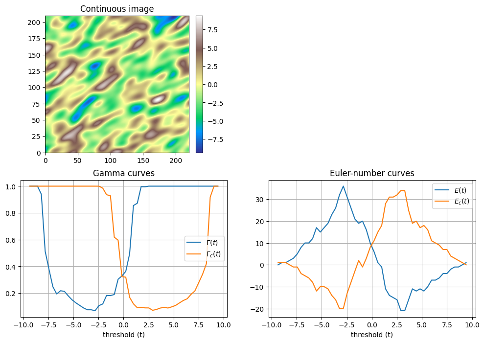
Connectivity analysis: Gamma and Euler number curves

Consider a continuous variable $v$ (continuous image) and for a threshold value $t$ the indicator variable defined as $I(t)(x) = 1 \iff v(x) \leqslant t$ .

Then, the Gamma value and the Euler number can be computed for the indicator variable $I(t)$ and for the complementary variable $I_c(t) = 1 - I(t)$ . By varying the threshold value $t$ , one obtain the curve $\Gamma(t)$ , $E(t)$ and $\Gamma_c(t)$ , $E_c(t)$ (for $I(t)$ and $I_c(t)$ resp.).

The functions geone.geosclassicinterface.imgConnectivityGammaCurves and geone.geosclassicinterface.imgConnectivityEulerNumberCurves computes theses curves. The threshold values considered are determined by the keyword arguments threshold_min, threshold_max and nthreshold: nthreshold equidistant values are considered, from threshold_min to threshold_max (i.e. numpy.linspace(threshold_min, threshold_max, nthreshold)). By default, threshold_min (resp. threshold_max) is set to the minimal (resp. maximal) value of the variable $v$ minus (resp. plus) 1.0e-10, and nthreshold to $50$ .

These functions return an array of shape (nthreshold, 3) with the threshold values in colunm of index 0, and the Gamma values and resp. Euler numbers for the variable $I$ in column of index 1 and for the variable $I_c$ in column of index 2.

The type of connectivity (keyword argument connect_type, see above) can be specified only for the function geone.geosclassicinterface.imgConnectivityGammaCurves.

Note that for both functions the input image must have only one variable.

For both functions, the number of threads used (keyword argument nthreads, see above) can be specified.

[10]:

# Compute gamma and Euler-number curves for the continuous image
gammat = gn.geosclassicinterface.imgConnectivityGammaCurves(im_cont)
eult = gn.geosclassicinterface.imgConnectivityEulerNumberCurves(im_cont)

# Display
plt.subplots(2,2,figsize=(12,8))

plt.subplot(2,2,2)
plt.axis('off')

plt.subplot(2,2,1)
gn.imgplot.drawImage2D(im_cont, cmap='terrain', title='Continuous image')

plt.subplot(2,2,3)
plt.plot(gammat[:,0], gammat[:,1], label='$\Gamma(t)$')
plt.plot(gammat[:,0], gammat[:,2], label='$\Gamma_c(t)$')
plt.xlabel('threshold (t)')
plt.grid()
plt.legend()
plt.title('Gamma curves')

plt.subplot(2,2,4)
plt.plot(eult[:,0], eult[:,1], label='$E(t)$')
plt.plot(eult[:,0], eult[:,2], label='$E_c(t)$')
plt.xlabel('threshold (t)')
plt.grid()
plt.legend()
plt.title('Euler-number curves')

plt.show()

<>:15: SyntaxWarning: invalid escape sequence '\G'
<>:16: SyntaxWarning: invalid escape sequence '\G'
<>:15: SyntaxWarning: invalid escape sequence '\G'
<>:16: SyntaxWarning: invalid escape sequence '\G'
/tmp/ipykernel_123504/2217170277.py:15: SyntaxWarning: invalid escape sequence '\G'
  plt.plot(gammat[:,0], gammat[:,1], label='$\Gamma(t)$')
/tmp/ipykernel_123504/2217170277.py:16: SyntaxWarning: invalid escape sequence '\G'
  plt.plot(gammat[:,0], gammat[:,2], label='$\Gamma_c(t)$')

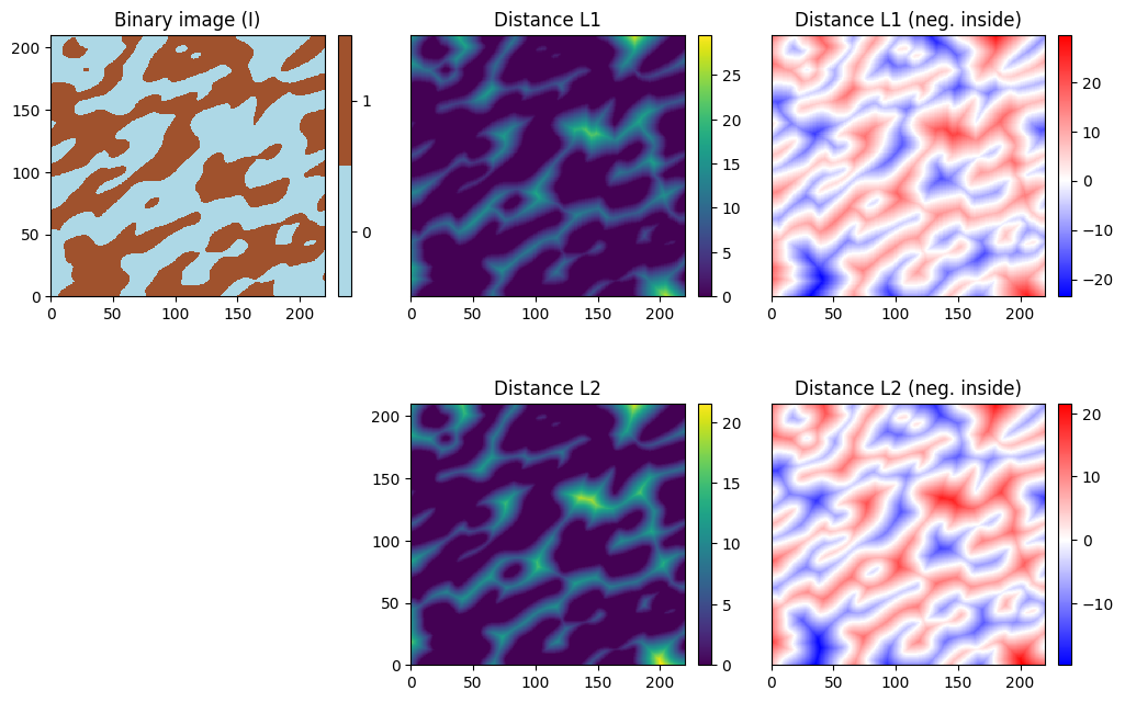
../_images/notebooks_ex_geosclassic_image_analysis_17_1.png

Other tools: distance to binary media

The function geone.geosclassicinterface.imgDistanceImagecomputes the distance to the set $S = \{v\neq 0\}$ , where $v$ is the variable of the input image, from every grid cell.

Distances $L_1$ and $L_2$ can be computed, this is specified by the keyword argument distance_type (string) which should be L1 or L2 (default). In addition, setting the keyword argument distance_negative to True, the distances (with a negative sign) from the interior cell of the set $S$ to its border are computed. By default, distance_negative=False (distance is zero for any cell in $S$ ).

This function launches a C program running in parallel, the number of threads used (keyword argument nthreads, see above) can be specified.

[11]:

# Compute distance L1 for the binary image
im_bin_dist_L1   = gn.geosclassicinterface.imgDistanceImage(im_bin, distance_type='L1', distance_negative=False)
im_bin_dist_L1_n = gn.geosclassicinterface.imgDistanceImage(im_bin, distance_type='L1', distance_negative=True)

# Compute distance L2 for the binary image
im_bin_dist_L2   = gn.geosclassicinterface.imgDistanceImage(im_bin, distance_type='L2', distance_negative=False)
im_bin_dist_L2_n = gn.geosclassicinterface.imgDistanceImage(im_bin, distance_type='L2', distance_negative=True)

# Display images
# Custom color map from blue (min) to white (value=0) to red (max)
# ... for im_bin_dist_L1_n
cmap1 = gn.customcolors.custom_cmap(
            ['blue', 'white', 'red'],
            vseq=[im_bin_dist_L1_n.val.min(), 0, im_bin_dist_L1_n.val.max()])
# ... for im_bin_dist_L2_n
cmap2 = gn.customcolors.custom_cmap(
            ['blue', 'white', 'red'],
            vseq=[im_bin_dist_L2_n.val.min(), 0, im_bin_dist_L2_n.val.max()])

plt.subplots(2,3,figsize=(12,8))

plt.subplot(2,3,1)
gn.imgplot.drawImage2D(im_bin, categ=True, categVal=[0,1], categCol=col_bin, title='Binary image (I)')

plt.subplot(2,3,2)
gn.imgplot.drawImage2D(im_bin_dist_L1, yticks=[], title='Distance L1')

plt.subplot(2,3,3)
gn.imgplot.drawImage2D(im_bin_dist_L1_n, cmap=cmap1, yticks=[], title='Distance L1 (neg. inside)')

plt.subplot(2,3,4)
plt.axis('off')

plt.subplot(2,3,5)
gn.imgplot.drawImage2D(im_bin_dist_L2, title='Distance L2')

plt.subplot(2,3,6)
gn.imgplot.drawImage2D(im_bin_dist_L2_n, cmap=cmap2, yticks=[], title='Distance L2 (neg. inside)')

plt.show()

../_images/notebooks_ex_geosclassic_image_analysis_19_0.png

GEONE - GEOSCLASSIC - Two-point statistics analysis of images

Import what is required

Remark

Generate a continuous image and a binary image (2D)

Basic two-point statistics

Function geone.geosclassicinterface.imgTwoPointStatisticsImage

Connectivity: geobody image

Function geone.geosclassicinterface.imgGeobodyImage

Connectivity analysis: ‘’connectogram’’

Function geone.geosclassicinterface.imgTwoPointStatisticsImage

Connectivity analysis: Gamma value and Euler number

Gamma value

Euler number

Function geone.geosclassicinterface.imgConnectivityGammaValue and

Function geone.geosclassicinterface.imgConnectivityEulerNumber

Connectivity analysis: Gamma and Euler number curves

Other tools: distance to binary media

Function `geone.geosclassicinterface.imgTwoPointStatisticsImage`

Function `geone.geosclassicinterface.imgGeobodyImage`

Function `geone.geosclassicinterface.imgTwoPointStatisticsImage`

Function `geone.geosclassicinterface.imgConnectivityGammaValue` and

Function `geone.geosclassicinterface.imgConnectivityEulerNumber`