GEONE - Variogram analysis and kriging for data in 1D

Interpolate a data set in 1D, using simple or ordinary kriging. Starting from a data set in 1D, the following is done:

basic exploratory analysis: variogram cloud / experimental variogram
fitting a covariance / variogram model, and cross-validation (LOO error)
interpolation by ordinary kriging (OK), simple kriging (SK)
sequential gaussian simulation (SGS) based on ordinary or simple kriging

Note: most of the tools illustrated below can also be used for data in 2D or 3D assuming omni-directional covariance / variogram models.

Import what is required

[1]:

import numpy as np
import matplotlib.pyplot as plt
import scipy
import time

# import package 'geone'
import geone as gn

[2]:

# Show version of python and version of geone
import sys
print(sys.version_info)
print('geone version: ' + gn.__version__)

sys.version_info(major=3, minor=13, micro=7, releaselevel='final', serial=0)
geone version: 1.3.1

Remark

The matplotlib figures can be visualized in interactive mode:

%matplotlib notebook: enable interactive mode
%matplotlib inline: disable interactive mode

Preparation - build a data set in 1D

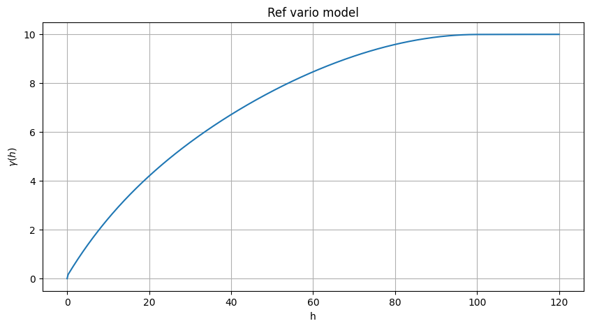
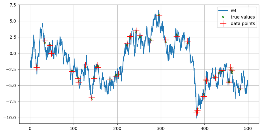
A data set in 1D is extracted from a Gaussian random field generated based on a known covariance model, called the reference model which will be considered as unknown further.

Note: see the notebook ``ex_general_multiGaussian.ipynb`` for available covariance models and examples.

[3]:

cov_model_ref = gn.covModel.CovModel1D(elem=[
    ('spherical', {'w':7., 'r':100}),   # elementary contribution
    ('exponential', {'w':2.9, 'r':50}), # elementary contribution
    ('nugget', {'w':0.1})               # elementary contribution
    ], name='ref model')

[4]:

cov_model_ref

[4]:

*** CovModel1D object ***
name = 'ref model'
number of elementary contribution(s): 3
elementary contribution 0
    type: spherical
    parameters:
        w = 7.0
        r = 100
elementary contribution 1
    type: exponential
    parameters:
        w = 2.9
        r = 50
elementary contribution 2
    type: nugget
    parameters:
        w = 0.1
*****

[5]:

# Plot reference variogram model
plt.figure(figsize=(10,5))
cov_model_ref.plot_model(vario=True)
plt.title('Ref vario model')
plt.show()

../_images/notebooks_ex_vario_analysis_data1D_1_7_0.png

Generate a gaussian random field in 1D (see function geone.grf.grf1D), and extract data points:

n: number of data points
x: location of data points (1-dimensional array of length n)
v: values at data points (1-dimensional array of length n)

[6]:

# Simulation grid (domain)
nx = 1000 # number of cells
sx = 0.5  # cell unit
ox = 0.0  # origin
# xmin, xmax = ox, ox + nx*sx # bounds of the simulation domain

# Reference simulation
np.random.seed(123)
ref = gn.grf.grf1D(cov_model_ref, nx, sx, ox, nreal=1) # 2d-array of shape 1 x nx

im_ref = gn.img.Img(nx, 1, 1, sx, 1., 1., ox, 0., 0., nv=1, val=ref) # fill image (Img class from geone.img)

# Extract n points from the reference simulation
n = 40
np.random.seed(987)
x = im_ref.xmin() + np.random.random(n) * (im_ref.xmax()-im_ref.xmin()) # random location in the grid
f = gn.img.Img_interp_func(im_ref, iy=0, iz=0) # function interpolating the image values
v_true = f(x) # value at x

# Add noise (Gaussian) to the values
v_err_std = 0.2
v = v_true + scipy.stats.norm.rvs(size=n, loc=0, scale=v_err_std)

[7]:

# Plot reference simulation and data points
plt.figure(figsize=(10,5))
plt.plot(im_ref.x(), ref[0], label='ref')
plt.plot(x, v_true, c='green', ls='', marker='x', markersize=5, label='true values')
plt.plot(x, v, c='red', ls='', marker='+', markersize=15, label='data points')
plt.grid()
plt.legend()
plt.show()

../_images/notebooks_ex_vario_analysis_data1D_1_10_0.png

Start from a data set in 1D

n: number of data points
x: 1-dimensional array of length n: locations of data points
v: 1-dimensional array of length n: values at data points

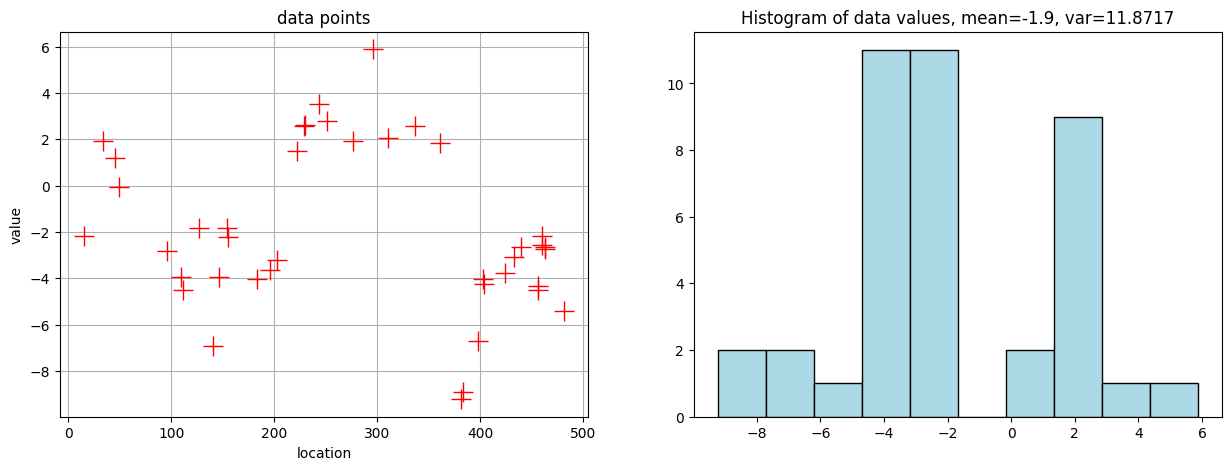
Visualise the data set and the histogram of values.

[8]:

plt.subplots(1,2,figsize=(15,5))
plt.subplot(1,2,1)
plt.plot(x, v, 'r+', markersize=15)
plt.xlabel('location')
plt.ylabel('value')
plt.grid()
plt.title('data points')

plt.subplot(1,2,2)
plt.hist(v, color='lightblue', edgecolor='black')
plt.title('Histogram of data values, mean={:.2g}, var={:2g}'.format(np.mean(v), np.var(v)))
plt.show()

../_images/notebooks_ex_vario_analysis_data1D_1_12_0.png

Variogram cloud

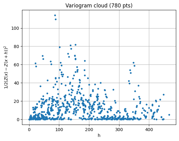
Compute the variogram cloud. The pair of the i-th and j-th data points gives the point $(h(i,j), g(i,j))$ in the variogram cloud, where

$h(i,j) = \vert\vert x(i)-x(j)\vert\vert$ is the distance between $x(i)$ and $x(j)$ (lag)
$g(i,j) = 1/2 \cdot (v(i)-v(j))^2)$ is the corresponding $\gamma$ value

The function geone.covModel.variogramCloud1D returns two 1-dimensional arrays h and g of same length npair containing the coordinates of the points in the variogram cloud. The maximal distance between two data points to be integrated in the variogram cloud can be specified by the keyword argument hmax. Note that a plot of the variogram cloud is made by default (keyword argument make_plot=True).

Note: for data in 2D or 3D, this function computes the omni-directional variogram cloud.

[9]:

h, g, npair = gn.covModel.variogramCloud1D(x, v)

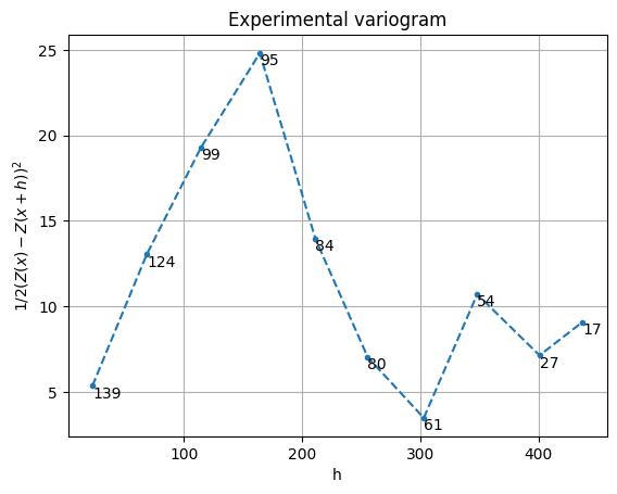
../_images/notebooks_ex_vario_analysis_data1D_1_14_0.png

Experimental variogram

Compute the experimental variogram. It is obtained from the variogram cloud by computing the mean points of variogram cloud points within vertical bands (classes for the lags). A class for a lag is an interval along the $h$ -axis.

The function geone.covModel.variogramExp1D returns three 1-dimensional arrays hexp, gexp, and cexp of same length (number of classes), where hexp and gexp contain the coordinates of the mean points of each class and cexp the number (counter) of points in each class.

The variogram cloud (if already computed) can be passed directly to the function geone.covModel.variogramExp1D via the keyword argument geone.covModel.variogramCloud: in this case, the arguments x, v, (and optional hmax) are not used. The classes can be defined in several ways: specifying the number of classes (ncla) / specifying the class centers (cla_center) / specifying the class length(s) (cla_length) (in particular overlapping classes are possible), see doc of the function). Note that a plot of the experimental variogram is made by default (keyword argument make_plot=True) with the counters displayed (keyword argument show_count=True).

Note: for data in 2D or 3D, this function computes the omni-directional experimental variogram.

[10]:

hexp, gexp, cexp = gn.covModel.variogramExp1D(x, v)
# hexp, gexp, cexp = gn.covModel.variogramExp1D(x, v, variogramCloud=(g, h, npair)) # equivalent (x, v not used)

../_images/notebooks_ex_vario_analysis_data1D_1_16_0.png

[11]:

hexp, gexp, cexp = gn.covModel.variogramExp1D(x, v, hmax=250, ncla=25)
# hexp, gexp, cexp = gn.covModel.variogramExp1D(x, v, cla_center=np.arange(5, 250, 10))

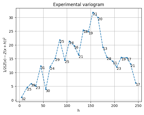
../_images/notebooks_ex_vario_analysis_data1D_1_17_0.png

Note that the function geone.covModel.plot_variogramExp1D allows to plot an experimental variogram (already computed): geone.covModel.plot_variogramExp1D(hexp, gexp, cexp) gives the plot above.

Model fitting

The function geone.covModelcovModel1D_fit allows to fit a covariance / variogram model in 1D to given data.

This function takes as first argument the location of the data points, as second argument the values at the data points, and at third argument a covariance model in 1D with given type of elementary contributions and with parameters to fit set to nan. It returns the optimal covariance model and the vector of optimal parameters.

This function is based on the function curve_fit from scipy.optimize module. It fits the curve of the variogram model to the points $(h, \gamma(h))$ , where $h$ is the lag between a pair of data points and $\gamma(h)$ is the half of the square of the difference of the values at these points (i.e. fit to the points of the variogram cloud). Hence, the fitting does not depend on the experimental variogram, i.e. on the choice of the classes for the lags.

The function geone.covModelcovModel1D_fit also takes the keyword argument hmax, which specifies the maximal distance between two data points to be integrated in the fitting. Note that a plot of the optimal model returned is made by default (keyword argument make_plot=True).

Note: for data in 2D or 3D, this function fits an omni-directional model.

[12]:

cov_model_to_optimize = gn.covModel.CovModel1D(
    elem=[('gaussian',    {'w':np.nan, 'r':np.nan}), # elementary contribution
          ('spherical',   {'w':np.nan, 'r':np.nan}), # elementary contribution
          ('exponential', {'w':np.nan, 'r':np.nan}), # elementary contribution
          ('nugget',      {'w':np.nan})              # elementary contribution
    ], name='')
try:
    cov_model_opt, popt = gn.covModel.covModel1D_fit(x, v, cov_model_to_optimize)
    plt.show()
except Exception as exc:
    print('ERROR:', exc)

ERROR: covModel1D_fit: fitting covariance model failed

Bounds for parameters to fit

Bounds for parameters to fit can be specified to avoid meaningless optimal parameters returned (e.g. negative weight or range). Such bounds are given to the function geone.covModelcovModel1D_fit (and then to the function curve_fit from scipy.optimize) via the keyword arguments bounds=(<array of lower bounds>, <array of upper bounds>), where the arrays of lower / upper bounds have the same length as the vector of parameters to fit, with the $i-$ th entry corresponding to the $i$ -th parameter to fit (set to nan) in the covariance model passed as third argument. Note also that the keyword argument p0 allows to specify a vector of initial parameters (see doc of function curve_fit).

[13]:

cov_model_to_optimize = gn.covModel.CovModel1D(
    elem=[('gaussian',    {'w':np.nan, 'r':np.nan}), # elementary contribution
          ('spherical',   {'w':np.nan, 'r':np.nan}), # elementary contribution
          ('exponential', {'w':np.nan, 'r':np.nan}), # elementary contribution
          ('nugget',      {'w':np.nan})              # elementary contribution
                ], name='')
cov_model_opt, popt = gn.covModel.covModel1D_fit(x, v, cov_model_to_optimize,# hmax=300,
                                                 bounds=([ 0,   0,  0,   0,  0,   0,  0],
                                                         [20, 300, 20, 300, 20, 300, 20]),
                                                 make_plot=False)
# bounds are given for:
#  index 0: parameter 'w' of gaussian contribution
#  index 1: parameter 'r' of gaussian contribution
#  index 2: parameter 'w' of spherical contribution
#  index 3: parameter 'r' of spherical contribution
#  index 4: parameter 'w' of exponential contribution
#  index 5: parameter 'r' of exponential contribution
#  index 6: parameter 'w' of nugget contribution

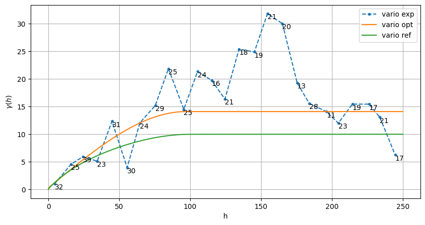
# Compare variogram exp. / variogram opt. / variogram ref
plt.figure(figsize=(10,5))
gn.covModel.plot_variogramExp1D(hexp, gexp, cexp, label='vario exp')
# hexp, gexp, cexp = gn.covModel.variogramExp1D(x, v, hmax=250, ncla=25, label='vario exp') # equiv.
cov_model_opt.plot_model(vario=True, hmax=250, label='vario opt')
cov_model_ref.plot_model(vario=True, hmax=250, label='vario ref')
plt.legend()
plt.show()
cov_model_opt

../_images/notebooks_ex_vario_analysis_data1D_1_22_0.png

[13]:

*** CovModel1D object ***
name = ''
number of elementary contribution(s): 4
elementary contribution 0
    type: gaussian
    parameters:
        w = 4.676321570099125e-08
        r = 80.7522710352472
elementary contribution 1
    type: spherical
    parameters:
        w = 13.843363090302038
        r = 97.1384629827674
elementary contribution 2
    type: exponential
    parameters:
        w = 2.9867267281186667e-13
        r = 74.79632981405173
elementary contribution 3
    type: nugget
    parameters:
        w = 0.26719882643054554
*****

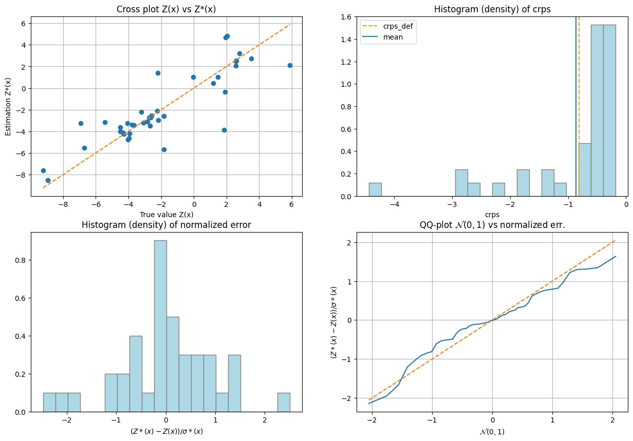
Cross-validation of covariance model by leave-one-out error

The function geone.covModel.cross_valid_loo performs a cross-validation test by leave-one-out (LOO) error. Given a data set, a covariance model and a kriging interpolator, the kriging estimate $Z^*(x)$ and standard deviation $\sigma^*(x)$ are computed at each data point $x$ , based on the data set without that data point $(x, Z(x))$ and the given covariance model.

The interpolator (function) used is passed by the keyword argument interpolator of the function geone.covModel.cross_valid_loo; the keyword argument interpolator_kwargs is a dictionary containing the keyword arguments that are passed to the function interpolator. By default:

interpolator=geone.covModel.krige, interpolator_kwargs=None: the function geone.covModel.krige is used as interpolator with default parameters, i.e. simple_kriging is used with mean value at the data points taken into account (i.e without the removed data point)

To use ordinary kriging as interpolator, set interpolator_kwargs={'method':'ordinary_kriging'} (see below details about the function geone.covModel.krige).

The continuous rank probability score (CRPS) is computed for each data point $x$ and defined as $\operatorname{crps}(F, x) = -\int_{-\infty}^{+\infty} \left(F(y)-\mathcal{1}\{y\geqslant x\}\right)^2 dy$ , where $F$ is the cumulative distribution function (CDF) of the prediction at $x$ , i.e. in this case, $F$ is the CDF of a normal distribution of mean $Z^*(x)$ and variance ${\sigma^*}^2(x)$ , $\mathcal{N}(Z^*(x), {\sigma^*}^2(x))$ . A “default” CRPS, corresponding to the unbiased prediction (i.e. $Z^*(x)=Z(x)$ ) with a variance given by the variance of the data values, is also computed.

Two statisic tests are performed on the normalized error $errn(x) = (Z^*(x)-Z(x))/\sigma^*(x)$ , which should approximately follows a standard normal distribution, $\mathcal{N}(0, 1)$ . Let $n$ be the number of data points.

Normal law test for mean of normalized error

With $\operatorname{mean}(errn)=1/n\sum_i errn(x[i])$ , the test computes:

the p-value: $\mathbb{P}\left(\vert Z\vert \geqslant \vert\operatorname{mean}(errn)\vert\right)$ , where $Z\sim\mathcal{N}(0, 1/n)$

Chi-square test for the sum of squares of normalized error

With $SSerrn = \sum_i errn(x[i])^2$ , the test computes:

the p-value: $\mathbb{P}\left(X \geqslant SSern\right)$ , where $X\sim\mathcal{\chi}^2_{n}$ , the chi-square distribution with $n$ degrees of freedom

Interpretation

A low p-value (e.g. below a significance level $\alpha=5\%$ ) means that the model should be rejected (falsely rejected with probability $\alpha$ ): the smaller the p-value, the more evidence there is to reject the model. Each test computes the p-value and the result (success/failure): the boolean success=(p-value > significance), which means that the model should be rejected when success=False with respect to the specified significance level.

Other statistics and plots

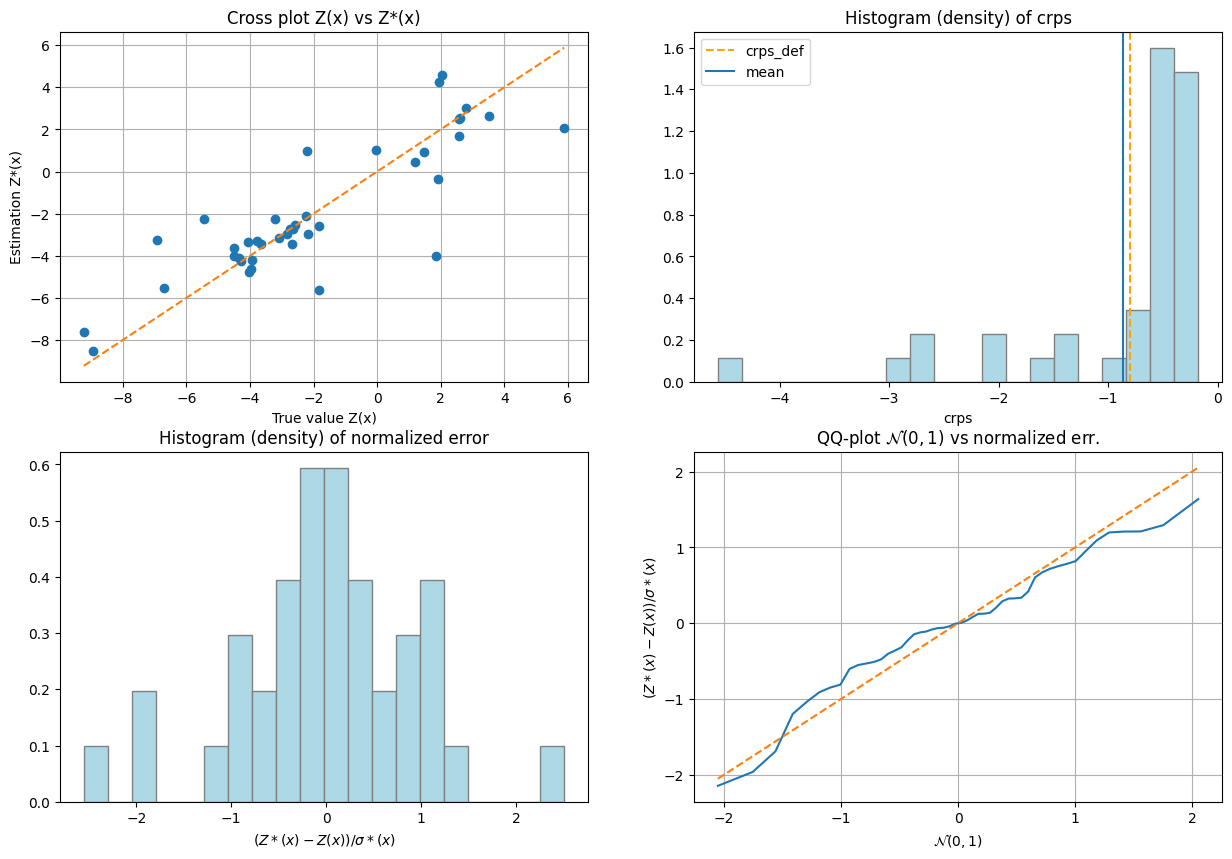
Specifying the keyword argument print_result=True (default), the function geone.covModel.cross_valid_loo prints the results of the statistics tests above, and some other statistics of the normalized error: the mean, standard deviation, skewness, excess kurtosis, to be compared with the standard normal distribution $\mathcal{N}(0,1)$ .

Specifying the keyword argument make_plot=True (default), the function geone.covModel.cross_valid_loo displays some plots about the cross-validation.

Returns

The function returns

cv_est, cv_std: respectively the cross-validation estimates $Z^*(x)$ and standard deviation $\sigma^*(x)$ for every data point (sequence / array of length $n$ )
crps, crps_def: the CRPS for every data points (array crps), and the “default” CRPS (of the unbiased prediction with a variance given by the variance of the data values) (float crps_def)
pvalue, success: respectively the p-values (floats) and the result (booleans) of each test (sequence of length $2$ )

[14]:

# Interpolation by simple kriging
cv_est1, cv_std1, crps1, crps_def1, pvalue1, success1 = gn.covModel.cross_valid_loo(
                                        x, v, cov_model_opt,
                                        interpolator=gn.covModel.krige,
                                        interpolator_kwargs={'method':'ordinary_kriging'},
                                        print_result=True, make_plot=True, figsize=(15,10), nbins=20)
plt.show()

----- CRPS (negative; the larger, the better) -----
   mean = -0.8601
   def. = -0.8052
----- 1) "Normal law test for mean of normalized error" -----
   p-value = 0.9614
   success = True (wrt significance level 0.05)
      (-> model has no reason to be rejected)
----- 2) "Chi-square test for sum of squares of normalized error" -----
   p-value = 0.6511
   success = True (wrt significance level 0.05)
      (-> model has no reason to be rejected)
----- Statistics of normalized error -----
   mean     = 0.007651 (should be close to 0)
   std      = 0.9486 (should be close to 1)
   skewness = -0.2492 (should be close to 0)
   excess kurtosis = 0.8769 (should be close to 0)

../_images/notebooks_ex_vario_analysis_data1D_1_24_1.png

[15]:

# Interpolation by ordinary kriging
cv_est2, cv_std2, crps2, crps_def2, pvalue2, success2 = gn.covModel.cross_valid_loo(
                                        x, v, cov_model_opt,
                                        interpolator=gn.covModel.krige, interpolator_kwargs={'method':'simple_kriging'},
                                        print_result=True, make_plot=True, figsize=(15,10), nbins=20)
plt.show()

----- CRPS (negative; the larger, the better) -----
   mean = -0.8607
   def. = -0.8052
----- 1) "Normal law test for mean of normalized error" -----
   p-value = 0.9955
   success = True (wrt significance level 0.05)
      (-> model has no reason to be rejected)
----- 2) "Chi-square test for sum of squares of normalized error" -----
   p-value = 0.6315
   success = True (wrt significance level 0.05)
      (-> model has no reason to be rejected)
----- Statistics of normalized error -----
   mean     = -0.0008858 (should be close to 0)
   std      = 0.9544 (should be close to 1)
   skewness = -0.2788 (should be close to 0)
   excess kurtosis = 0.9001 (should be close to 0)

../_images/notebooks_ex_vario_analysis_data1D_1_25_1.png

[16]:

# Comparison of cross-validation with simple kriging and ordinary kriging
plt.subplots(1, 2, figsize=(15,5))

plt.subplot(1,2,1)
# plt.plot(cv_est1, cv_est2, marker='+', ls='')
# plt.plot([np.min(cv_est1), np.max(cv_est1)], [np.min(cv_est1), np.max(cv_est1)], c='orange', ls='dashed')
# plt.axis('equal')
# plt.xlabel('Estimate SK')
# plt.ylabel('Estimate OK')
plt.plot(v, cv_est1, c='green', marker='+', ls='', label='SK')
plt.plot(v, cv_est2, c='purple', marker='x', ls='', label='OK')
plt.plot([np.min(v), np.max(v)], [np.min(v), np.max(v)], c='orange', ls='dashed')
plt.axis('equal')
plt.xlabel('Estimate SK')
plt.ylabel('Estimate OK')
plt.legend()
plt.grid()
plt.title('Comparison of CV estimates with SK and OK')

plt.subplot(1,2,2)
plt.plot(cv_std1, cv_std2, marker='+', ls='')
plt.plot([np.min(cv_std1), np.max(cv_std1)], [np.min(cv_std1), np.max(cv_std1)], c='orange', ls='dashed')
plt.axis('equal')
plt.xlabel('St. dev. SK')
plt.ylabel('St. dev. OK')
plt.title('Comparison of CV st. dev. with SK and OK')
plt.grid()
plt.show()

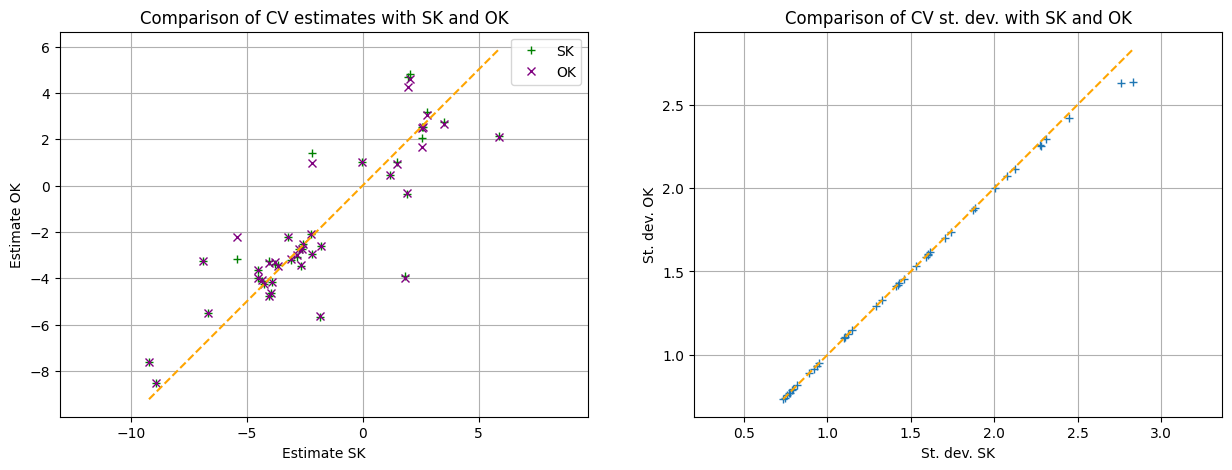
../_images/notebooks_ex_vario_analysis_data1D_1_26_0.png

If one test failed (or if the covariance model does not display the desired shape), the covariance model should be rejected and the search for a convenient covariance model be pursued.

Covariance model fitted on data with error

When data error (standard deviation of a zero-mean Gaussian) distribution is considered, a nugget effect of the (mean) of the error variance should be substracted from the covariance model used.

Thus, to avoid negative nugget, we can impose a lower bound for the nugget contribution when fitting the model.

[17]:

# ... elementary contribution of index 3 is the nugget
cov_model_opt.elem[3]

[17]:

('nugget', {'w': np.float64(0.26719882643054554)})

[18]:

# Substract variance error from the nugget
try:
    cov_model_opt.add_w(-v_err_std**2, elem_ind=3)
except:
    print('Ensure minimal nugget of variance error in the fitted covariance model')

[19]:

cov_model_opt.elem[3]

[19]:

('nugget', {'w': np.float64(0.22719882643054554)})

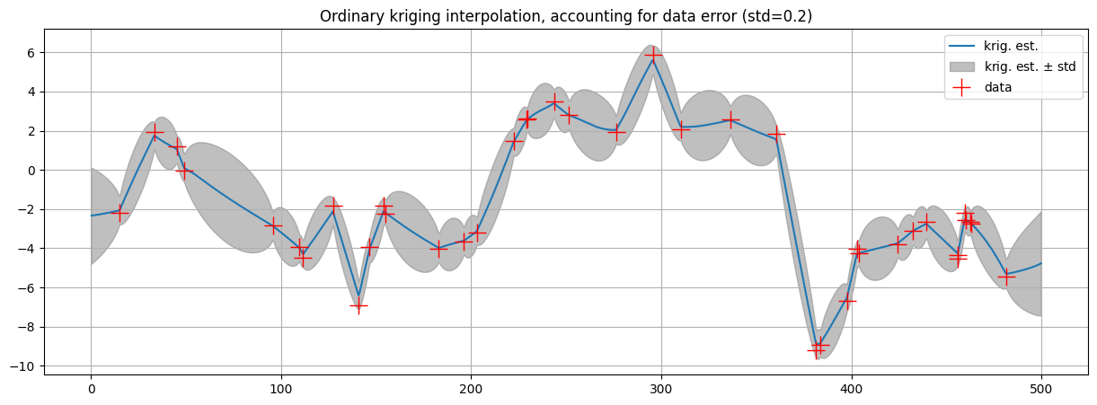
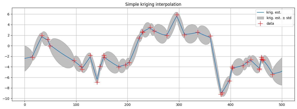
Data interpolation by (simple or ordinary) kriging: function `geone.covModel.krige`

The function geone.covModel.krige(x, v, xu, cov_model, **kwargs) return the kriging estimates and standard deviation at location xu, given the data points located at x with value v and the covariance model cov_model. Type of kriging is determined by the keyword argument method:

method='simple_kriging': simple kriging is used, with the mean according to the keyword argument mean (mean of the data values is used if mean=None)
method='ordinary_kriging' (default): ordinary kriging is used (the keyword argument mean must be None in this case)

Furthermore, the following parameters (keyword arguments) are available:

use_unique_neighborhood: boolean
- if True: kriging is done with a unique neighborhood (i.e. accounting for all data points)
- if False (default): kriging is done by accounting for (a limited number of) data points within a search ellipsoid centered at the estimated point (see parameters searchRadius, searchRadiusRelative and nneighborMax)
searchRadius : float or None; if specified (not None), radius of the search ellipsoid in any direction
searchRadiusRelative: float, used only if searchRadius=None, then with $r_i$ is the range of the covariance model along the direction $i$ , the radius of the search ellipsoid is set to searchRadiusRelative $\cdot$ $r_i$ in that direction
nneighborMax : int, maximal number of data points taken into account for kriging

For data in d dimension (here d=1):

x: 2-dimensional array of shape (n, d) or 1-dimensional array of length n, location of data points
v: 1-dimensional array of length n, values at data points
xu: 2-dimensional array of shape (m, d) or 1-dimensional array of length m, location of points where the interpolation is done

In return:

vu: 1-dimensional array of length m, kriging estimates at location xu
vu_std: 1-dimensional array of length m, kriging standard deviation at location xu

[20]:

# Define points xu where to interpolate
# ... location of the 1D-grid used to build the data set (but it could be different)
xu = ox + (np.arange(nx)+0.5)*sx

# Simple kriging
vu, vu_std = gn.covModel.krige(x, v, xu, cov_model_opt, v_err_std=v_err_std, method='ordinary_kriging', use_unique_neighborhood=True)
# vu:     1-dimensional array, kriging estimates at location xu
# vu_std: 1-dimensional array, kriging standard deviation at location xu

# Plot
plt.figure(figsize=(15,5))
plt.plot(xu, vu, label='krig. est.')
plt.fill_between(xu, vu-vu_std, vu+vu_std, color='gray', alpha=0.5, label=r'krig. est. $\pm$ std')
plt.plot(x, v, 'r+', markersize=15, label='data')
plt.grid()
plt.legend()
plt.title(f'Ordinary kriging interpolation, accounting for data error (std={v_err_std})')
plt.show()

../_images/notebooks_ex_vario_analysis_data1D_1_33_0.png

[21]:

# Define points xu where to interpolate
# ... location of the 1D-grid used to build the data set (but it could be different)
xu = ox + (np.arange(nx)+0.5)*sx

# Ordinary kriging
vu, vu_std = gn.covModel.krige(x, v, xu, cov_model_opt, v_err_std=v_err_std, method='simple_kriging', use_unique_neighborhood=True)
# vu:     1-dimensional array, kriging estimates at location xu
# vu_std: 1-dimensional array, kriging standard deviation at location xu

# Plot
plt.figure(figsize=(15,5))
plt.plot(xu, vu, label='krig. est.')
plt.fill_between(xu, vu-vu_std, vu+vu_std, color='gray', alpha=0.5, label=r'krig. est. $\pm$ std')
plt.plot(x, v, 'r+', markersize=15, label='data')
plt.grid()
plt.legend()
plt.title('Simple kriging interpolation')
plt.show()

../_images/notebooks_ex_vario_analysis_data1D_1_34_0.png

Simulation based on simple or ordinary kriging: function `geone.covModel.sgs`

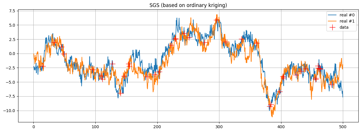
The function geone.covModel.sgs(x, v, xu, cov_model, **kwargs) performs sequential gaussian simulation (SGS) based on simple or ordinary kriging, it returns realizations at location xu, given the data points located at x with value v and the covariance model cov_model. Simulation uses a limited neighorhood, i.e. a limited number of data points and previously simulated points are taken into account to solve the kriging system for simulating the value at a point, which is drawn in a normal law of mean equal to the kriged value and variance equal to the kriging variance.

Number of realizations is set by the keyword argument nreal. The type of kriging is set by the keyword argument method, the maximal number of neighbors and the search ellipsoid by searchRadius, searchRadiusRelative and nneighborMax, as for the function geone.covModel.krige (see above); note that unique neighborhood is not possible for simulation.

For data in 1D:

x: 2-dimensional array of shape (n, 1) or 1-dimensional array of length n, location of data points
v: 1-dimensional array of length n, values at data points
xu: 2-dimensional array of shape (m, 1) or 1-dimensional array of length m, location of points where the simulation is done

In return:

vu: 2-dimensional array of shape (nreal, m), each row is a realization of the simulated values at xu

Launching multiple processes for multi-realizations of SGS

The function geone.covModel.sgs_mp launches multiple processes, allowing to generate multiple realizations in parallel.

The function geone.covModel.sgs_mp has the same parameters as the function geone.covModel.sgs, plus the parameter nproc, determining the number of parallel processes. This function will run nproc parallel processes (parallel calls of function geone.covModel.sgs). The ensemble of realizations (specified by nreal) is distributed in a balanced way over the process(es). For the parameter nproc, a negative number (or zero) (by default nproc=-1), nproc = -n $\leqslant$ 0, can be specified to use the total number of cpu(s) of the system except n; nproc is finally at maximum equal to nreal but at least 1 by applying:

if nproc $\geqslant$ 1, then nproc = max(min(nproc, nreal), 1) is used
if nproc = -n $\leqslant$ 0, then nproc = max(min(nmax-n, nreal), 1) is used, where nmax is the total number of cpu(s) of the system (retrieved by os.cpu_count())

[22]:

# Define points xu where to simulate
sim_xu = xu

# SGS based on simple kriging
nreal = 2
np.random.seed(321)
t1 = time.time()
sim_vu = gn.covModel.sgs(x, v, sim_xu, cov_model_opt, v_err_std=v_err_std, method='ordinary_kriging', nreal=nreal)
# sim_vu:   2-dimensional array of shape (nreal, len(sim_xu)), each row is a realization
#           (simulated values at locations sim_xu)
t2 = time.time()
print('Elapsed time: {:.2g} sec'.format(t2-t1))

# Plot
plt.figure(figsize=(15,5))
plt.plot(sim_xu, sim_vu[0], label='real #0')
plt.plot(sim_xu, sim_vu[1], label='real #1')
plt.plot(x, v, 'r+', markersize=15, label='data')
plt.grid()
plt.legend()
plt.title('SGS (based on ordinary kriging)')
plt.show()

Elapsed time: 0.59 sec

../_images/notebooks_ex_vario_analysis_data1D_1_36_1.png

Kriging estimation and simulation in a grid

The functions above (gn.covModel.krige and gn.covModel.sgs[_mp]) should not be used for kriging and SGS in a regular grid. There are dedicated functions that should be used instead (much faster for large grid (in 2D or 3D)), in the module geone.geosclassicinterface (see notebooks ex_geosclassic_*.ipynb), and the module geone.grf (see notebooks ex_grf_*.ipynb).

A brief description is given here:

geone.geosclassicinterface.estimate: estimation (kriging) in a grid
geone.geosclassicinterface.simulate: simulation (SGS) in a grid
geone.grf.krige<d>D: estimation (kriging) in a <d>-dimensional grid
geone.grf.grf<d>D: simulation (SGS) in a <d>-dimensional grid

Note: the functions of the module ``geone.grf`` are based on “Fast Fourier Transform” and allow for simple kriging only, and do not handle error on data or inequality data.

Wrapper

The function geone.multiGaussian.multiGaussianRun can be used as a wrapper; with keyword arguments:

mode='estimation', algo='classic': wrapper for geone.geosclassicinterface.estimate
mode='simulation', algo='classic': wrapper for geone.geosclassicinterface.simulate
mode='estimation', algo='fft': wrapper for geone.grf.krige<d>D
mode='simulation', algo='fft': wrapper for geone.grf.grf<d>D

where the dimension <d> is automatically detected. Note also that the function geone.multiGaussian.multiGaussianRun allows to choose the “format” of the output by the keyword argument output_mode:

output_mode='array': an numpy array is returned
output_mode='img': an “image” (class geone.img.Img) is returned

Examples

Estimation using the function `geone.covModel.krige`

[23]:

t1 = time.time()
vu, vu_std = gn.covModel.krige(x, v, xu, cov_model_opt, v_err_std=v_err_std, method='simple_kriging', use_unique_neighborhood=True)
t2 = time.time()
print('Elapsed time: {:.2g} sec'.format(t2-t1))

Elapsed time: 0.0057 sec

Estimation using the function `geone.grf.krige1D`

Via the function geone.multiGaussian.multiGaussianRun, with keyword arguments mode='estimation', algo='fft'.

[24]:

t1 = time.time()
vu_grf, vu_std_grf = gn.multiGaussian.multiGaussianRun(
                        cov_model_opt, nx, sx, ox,
                        x=x, v=v,
                        mode='estimation', algo='fft', output_mode='array')
# # Or
# vu_grf, vu_std_grf = gn.grf.krige1D(
#                         cov_model_opt, nx, sx, ox,
#                         x=x, v=v)
t2 = time.time()
print('Elapsed time: {:.2g} sec'.format(t2-t1))

krige1D: compute circulant embedding...
krige1D: embedding dimension: 2048
krige1D: compute FFT of circulant matrix...
krige1D: compute covariance matrix (rAA) for conditioning locations...
krige1D: compute covariance matrix (rBA) for non-conditioning / conditioning locations...
krige1D: compute rBA * rAA^(-1)...
krige1D: compute kriging estimates...
krige1D: compute kriging standard deviation ...
Elapsed time: 0.017 sec

Estimation using the function `geone.geosclassicinterface.estimate`

Via the function geone.multiGaussian.multiGaussianRun, with keyword arguments mode='estimation', algo='classic'.

[25]:

t1 = time.time()
vu_gci, vu_std_gci = gn.multiGaussian.multiGaussianRun(
                        cov_model_opt, nx, sx, ox, x=x, v=v,
                        mode='estimation', algo='classic', output_mode='array',
                        v_err_std=v_err_std,
                        method='simple_kriging', use_unique_neighborhood=True,
                        nthreads=8)
# # Or
# estim_gci = gn.geosclassicinterface.estimate(
#                         cov_model_opt, nx, sx, ox,
#                         x=x, v=v,
#                         v_err_std=v_err_std,
#                         method='simple_kriging', use_unique_neighborhood=True)
# vu_gci, vu_std_gci = estim_gci['image'].val[:,0,0,:]
t2 = time.time()
print('Elapsed time: {:.2g} sec'.format(t2-t1))

estimate: pre-process data done: final number of data points : 40, inequality data points: 0
estimate: computational resources: nthreads = 8, nproc_sgs_at_ineq = 8
estimate: (Step 1) no inequality data
estimate: (Step 2) set new dataset gathering data and inequality data locations...
estimate: (Step 3) do kriging at the center of grid cells containing at least one data point...
estimate: (Step 4) do kriging on the grid (at cell centers) using data points at cell centers...
estimate: call `run_MPDSOMPGeosClassicSim` [1 process of 8 thread(s) (OpenMP)] ...
estimate: `run_MPDSOMPGeosClassicSim` [1 process] complete
Elapsed time: 0.021 sec

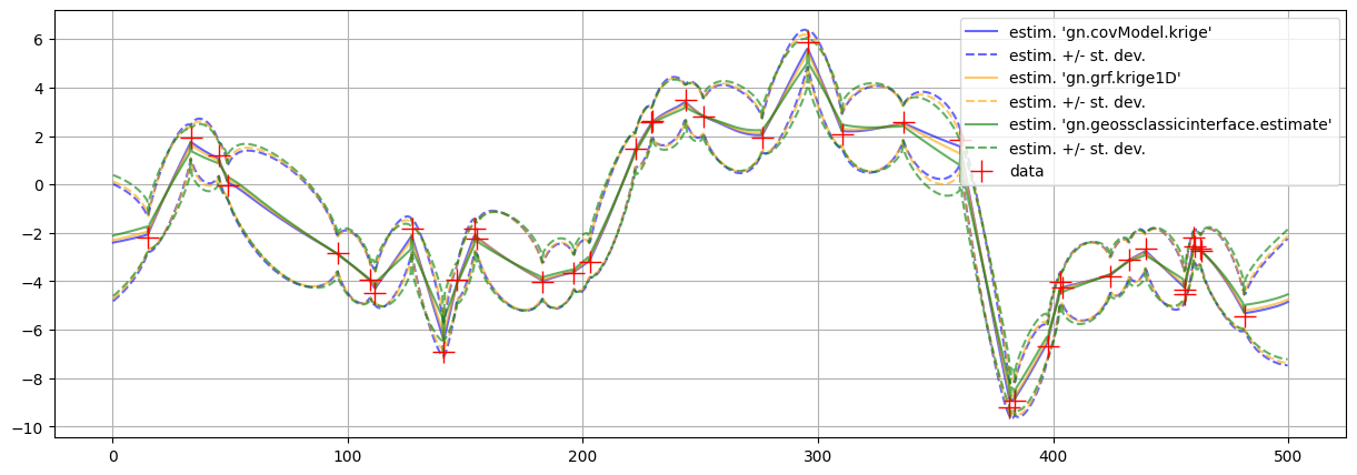
Plot results of estimation

[26]:

# Plot
plt.figure(figsize=(15,5))
plt.plot(xu, vu, color='blue', ls='solid', alpha=.6, label="estim. 'gn.covModel.krige'")
plt.plot(xu, vu + vu_std, color='blue', ls='dashed', alpha=.6, label='estim. +/- st. dev.')
plt.plot(xu, vu - vu_std, color='blue', ls='dashed', alpha=.6)

plt.plot(xu, vu_grf, color='orange', ls='solid', alpha=.6, label="estim. 'gn.grf.krige1D'")
plt.plot(xu, vu_grf + vu_std_grf, color='orange', ls='dashed', alpha=.6, label='estim. +/- st. dev.')
plt.plot(xu, vu_grf - vu_std_grf, color='orange', ls='dashed', alpha=.6)

plt.plot(xu, vu_gci, color='green', ls='solid', alpha=.6, label="estim. 'gn.geossclassicinterface.estimate'")
plt.plot(xu, vu_gci + vu_std_gci, color='green', ls='dashed', alpha=.6, label='estim. +/- st. dev.')
plt.plot(xu, vu_gci - vu_std_gci, color='green', ls='dashed', alpha=.6)

plt.plot(x, v, 'r+', markersize=15, label='data')
plt.grid()
plt.legend()
plt.show()

../_images/notebooks_ex_vario_analysis_data1D_1_46_0.png

[27]:

print("Peak-to-peak estimation 'gn.covModel.krige - gn.grf.krige1D'                   = {}".format(np.ptp(vu - vu_grf)))
print("Peak-to-peak estimation 'gn.covModel.krige - gn.geosclassicinterface.estimate' = {}".format(np.ptp(vu - vu_gci)))
print("Peak-to-peak estimation 'gn.grf.krige1D    - gn.geosclassicinterface.estimate' = {}".format(np.ptp(vu_grf - vu_gci)))
print("Peak-to-peak st. dev.   'gn.covModel.krige - gn.grf.krige1D'                   = {}".format(np.ptp(vu_std - vu_std_grf)))
print("Peak-to-peak st. dev.   'gn.covModel.krige - gn.geosclassicinterface.estimate' = {}".format(np.ptp(vu_std - vu_std_gci)))
print("Peak-to-peak st. dev.   'gn.grf.krige1D    - gn.geosclassicinterface.estimate' = {}".format(np.ptp(vu_std_grf - vu_std_gci)))

Peak-to-peak estimation 'gn.covModel.krige - gn.grf.krige1D'                   = 0.6202799930551004
Peak-to-peak estimation 'gn.covModel.krige - gn.geosclassicinterface.estimate' = 1.596589893876738
Peak-to-peak estimation 'gn.grf.krige1D    - gn.geosclassicinterface.estimate' = 0.9905537155280293
Peak-to-peak st. dev.   'gn.covModel.krige - gn.grf.krige1D'                   = 0.11695451499708254
Peak-to-peak st. dev.   'gn.covModel.krige - gn.geosclassicinterface.estimate' = 0.2982567859129016
Peak-to-peak st. dev.   'gn.grf.krige1D    - gn.geosclassicinterface.estimate' = 0.25057269986451836

Conditional simulation using the function `geone.covModel.sgs`

[28]:

np.random.seed(293)

# SGS based on simple kriging
nreal = 200 # only!
t1 = time.time()
sim_vu = gn.covModel.sgs(x, v, xu, cov_model_opt, v_err_std=v_err_std, method='ordinary_kriging', nreal=nreal)
t2 = time.time()
print('Elapsed time: {:.2g} sec'.format(t2-t1))

Elapsed time: 49 sec

Conditional simulation using the function `geone.grf.grf1D`

Via the function geone.multiGaussian.multiGaussianRun, with keyword arguments mode='simulation', algo='fft'.

[29]:

np.random.seed(293)

t1 = time.time()
nreal = 1000
sim_grf = gn.multiGaussian.multiGaussianRun(
                        cov_model_opt, nx, sx, ox,
                        x=x, v=v,
                        mode='simulation', algo='fft', output_mode='array',
                        nreal=nreal)
# # Or:
# sim_grf = gn.grf.grf1D(
#                         cov_model_opt, nx, sx, ox,
#                         x=x, v=v,
#                         nreal=nreal)
t2 = time.time()
print('Elapsed time: {:.2g} sec'.format(t2-t1))

grf1D: do preliminary computation...
grf1D: compute circulant embedding...
grf1D: embedding dimension: 2048
grf1D: compute FFT of circulant matrix...
grf1D: treatment of conditioning data...
grf1D: compute covariance matrix (rAA) for conditioning locations...
grf1D: compute index in the embedding grid for non-conditioning / conditioning locations...
Elapsed time: 9.6 sec

Conditional simulation using the function `geone.geosclassicinterface.simulate`

Via the function geone.multiGaussian.multiGaussianRun, with keyword arguments mode='simulation', algo='classic', and specifying the computational resources (nproc and nthreads_per_proc).

[30]:

np.random.seed(293)

t1 = time.time()
nreal = 1000
sim_gci = gn.multiGaussian.multiGaussianRun(
                        cov_model_opt, nx, sx, ox,
                        x=x, v=v,
                        mode='simulation', algo='classic', output_mode='array',
                        v_err_std=v_err_std,
                        method='simple_kriging',
                        nreal=nreal,
                        nproc=2, nthreads_per_proc=4)
# # Or:
# sim_gci = gn.geosclassicinterface.simulate(
#                         cov_model_opt, nx, sx, ox,
#                         x=x, v=v,
#                         v_err_std=v_err_std,
#                         method='simple_kriging',
#                         nreal=nreal,
#                         nproc=2, nthreads_per_proc=4)
# sim_gci = sim_gci['image'].val[:,0,0,:]
t2 = time.time()
print('Elapsed time: {:.2g} sec'.format(t2-t1))

simulate: pre-process data done: final number of data points : 40, inequality data points: 0
simulate: computational resources: nproc = 2, nthreads_per_proc = 4, nproc_sgs_at_ineq = 8
simulate: (Step 1) no inequality data
simulate: (Step 2) set new dataset gathering data and inequality data locations...
simulate: (Step 3) do kriging at the center of grid cells containing at least one data point...
simulate: (Step 4) do sgs (1000 realizations) on the grid (at cell centers) using data points at cell centers...
simulate: call `run_MPDSOMPGeosClassicSim` [2 process(es) of 4 thread(s) (OpenMP)] ...
simulate: `run_MPDSOMPGeosClassicSim` [2 process(es)] complete
Elapsed time: 1.4 sec

Plot some realizations and compare to the reference simulation

[31]:

sim_vu_mean = sim_vu.mean(axis=0)
sim_vu_std  = sim_vu.std(axis=0)

sim_grf_mean = sim_grf.mean(axis=0)
sim_grf_std  = sim_grf.std(axis=0)

sim_gci_mean = sim_gci.mean(axis=0)
sim_gci_std  = sim_gci.std(axis=0)

[32]:

# Plot
plt.figure(figsize=(15,5))

for i in range(1):
    if i == 0:
        label = "sim. 'gn.covModel.sgs' (sgs)"
    else:
        label = None
    plt.plot(xu, sim_gci[i], color='orange', alpha=.2, label=label)

for i in range(1):
    if i == 0:
        label = "sim. 'gn.grf.grf1D' (grf)"
    else:
        label = None
    plt.plot(xu, sim_grf[i], color='green', alpha=.2, label=label)

for i in range(1):
    if i == 0:
        label = "sim. 'gn.geosclassicinterface.simulate' (gci)"
    else:
        label = None
    plt.plot(xu, sim_gci[i], color='purple', alpha=.2, label=label)

plt.plot(xu, sim_vu_mean, color='orange', ls='dashed', label=f'sgs mean ({200} real.)')
plt.fill_between(xu, sim_vu_mean-sim_vu_std, sim_vu_mean+sim_vu_std, color='orange', alpha=0.2, label=r'sgs mean $\pm$ std')

plt.plot(xu, sim_grf_mean, color='green', ls='dashed', label=f'grf mean ({nreal} real.)')
plt.fill_between(xu, sim_grf_mean-sim_grf_std, sim_grf_mean+sim_grf_std, color='green', alpha=0.2, label=r'grf mean $\pm$ std')

plt.plot(xu, sim_gci_mean, color='purple', ls='dashed', label=f'gci mean ({nreal} real.)')
plt.fill_between(xu, sim_gci_mean-sim_gci_std, sim_gci_mean+sim_gci_std, color='purple', alpha=0.2, label=r'gci mean $\pm$ std')

# plt.plot(xu, vu, color='lightblue', ls='dashed', label='krig. estim.')
# plt.fill_between(xu, vu-vu_std, vu+vu_std, color='blue', alpha=0.2, label=r'krig. estim. $\pm$ std')

plt.plot(xu, ref[0], color='blue', lw=.5, label='ref. sim')

plt.plot(x, v, 'r+', markersize=15, label='data')

plt.grid()
plt.legend(loc='upper right')
plt.show()

../_images/notebooks_ex_vario_analysis_data1D_1_56_0.png