GEONE - Variogram analysis and kriging for data in 3D (omni-directional)
Interpolate a data set in 3D, using ordinary kriging. Starting from a data set in 3D, the following is done:
basic exploratory analysis: variogram cloud / experimental variogram
fitting a covariance / variogram model, and cross-validation (LOO error)
interpolation by ordinary kriging (OK), simple kriging (SK)
sequential gaussian simulation (SGS) based on ordinary or simple kriging
Import what is required
[1]:
import numpy as np
import matplotlib.pyplot as plt
import pyvista as pv
import time

# import package 'geone'
import geone as gn
[2]:
# Show version of python and version of geone
import sys
print(sys.version_info)
print('geone version: ' + gn.__version__)
sys.version_info(major=3, minor=13, micro=7, releaselevel='final', serial=0)
geone version: 1.3.1
[3]:
pv.set_jupyter_backend('static') # static plots
# pv.set_jupyter_backend('trame')  # 3D-interactive plots
Preparation - build a data set in 3D
A data set in 3D is extracted from a Gaussian random field generated based on a known covariance model, called the reference model which will be considered as unknown further.
Define a (isotropic) reference covariance model in 1D (class geone.covModel.CovModel1D), used as omni-directional in 3D.
Note: see the notebook ``ex_general_multiGaussian.ipynb`` for available covariance models and examples.
[4]:
cov_model_ref = gn.covModel.CovModel1D(elem=[
    ('spherical', {'w':9.5, 'r':15.}), # elementary contribution (same ranges: isotropic)
    ('nugget', {'w':0.5})                       # elementary contribution
    ], name='ref model (isotropic)')
[5]:
cov_model_ref
[5]:
*** CovModel1D object ***
name = 'ref model (isotropic)'
number of elementary contribution(s): 2
elementary contribution 0
    type: spherical
    parameters:
        w = 9.5
        r = 15.0
elementary contribution 1
    type: nugget
    parameters:
        w = 0.5
*****
[6]:
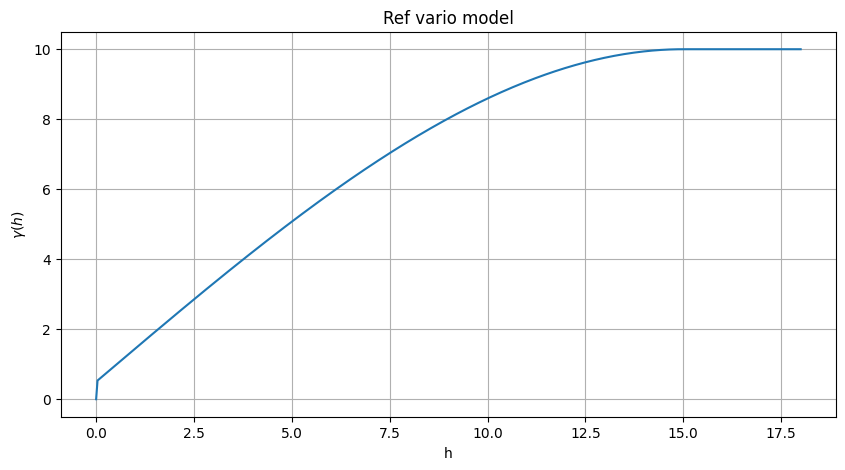
# Plot reference variogram model
plt.figure(figsize=(10,5))
cov_model_ref.plot_model(vario=True)
plt.title('Ref vario model')
plt.show()
Generate a gaussian random field in 3D (see function geone.grf.grf3D), and extract data points:
n: number of data pointsx: location of data points (2-dimensional array of shape(n, 3), each row is a point)v: values at data points (1-dimensional array of lengthn)
[7]:
# Simulation grid (domain)
nx, ny, nz = 65, 64, 60     # number of cells
sx, sy, sz = 0.5, 0.5, 0.5  # cell unit
ox, oy, oz = 0.0, 0.0, 0.0  # origin

# Reference simulation
np.random.seed(123)
ref = gn.grf.grf3D(cov_model_ref, (nx, ny, nz), (sx, sy, sz), (ox, oy, oz), nreal=1)
    # 4d-array of shape 1 x nz x ny x nx

im_ref = gn.img.Img(nx, ny, nz, sx, sy, sz, ox, oy, oz, nv=1, val=ref)

# Extract n points from the reference simulation
n = 150 # number of data points
# --- Choose 1. or 2. below ---
# # 1. Sampling the image
# ps = gn.img.sampleFromImage(im_ref, n, seed=234)
# # Data points and data value
# x = np.array((ps.x(), ps.y(), ps.z())).T
# v = ps.val[3]
# # Optionally: move points in the grid cells randomly, and add noise to values
# x[:, 0] = x[:, 0] + (np.random.random(n)-0.5)* im_ref.sx
# x[:, 1] = x[:, 1] + (np.random.random(n)-0.5)* im_ref.sy
# x[:, 2] = x[:, 2] + (np.random.random(n)-0.5)* im_ref.sz
# v = v + (np.random.random(n)-0.5)* 1.e-1

# 2. Using the function interpolating the image values
f = gn.img.Img_interp_func(im_ref)
np.random.seed(658)
x1 = im_ref.xmin() + np.random.random(n) * (im_ref.xmax()-im_ref.xmin())
x2 = im_ref.ymin() + np.random.random(n) * (im_ref.ymax()-im_ref.ymin())
x3 = im_ref.zmin() + np.random.random(n) * (im_ref.zmax()-im_ref.zmin())
x = np.array((x1, x2, x3)).T
v = f(x)
# ----- #
[8]:
# Preparation for plotting reference simulation and data points

# Color settings
cmap = 'terrain'

cmin = im_ref.vmin()[0] # min value in ref
cmax = im_ref.vmax()[0] # max value in ref

# Get colors for conditioning data according to their value and color settings
data_points_col = gn.imgplot.get_colors_from_values(v, cmap=cmap, cmin=cmin, cmax=cmax)

# Set points to be plotted
data_points = pv.PolyData(x)
data_points['colors'] = data_points_col
[9]:
# Plot reference simulation and data points

# Plot "interactive in pop-up window" or "inline" (comment the undesired one) ...
# ... interactive (after closing the pop-up window, the position of the camera is retrieved in output)
#pp = pv.Plotter(shape=(1,2), notebook=False)
# ... inline
pp = pv.Plotter(shape=(1,2))

pp.subplot(0, 0)
gn.imgplot3d.drawImage3D_volume(
    im_ref,
    plotter=pp,
    cmap=cmap, cmin=cmin, cmax=cmax,
    show_bounds=True, # show axes and ticks around the 3D box
    text='Ref') # title

pp.subplot(0, 1)
gn.imgplot3d.drawImage3D_slice(
    im_ref,
    plotter=pp,
    slice_normal_x=ox+0.5*sx,
    slice_normal_y=oy+(ny-0.5)*sy,
    slice_normal_z=oz+0.5*sz,
    cmap=cmap, cmin=cmin, cmax=cmax,
    show_bounds=True, # show axes and ticks around the 3D box
    scalar_bar_kwargs={'title':''}, # distinct title in each subplot for correct display!
    text='Ref and data points')

pp.add_mesh(data_points, rgb=True, point_size=12., render_points_as_spheres=True)

pp.link_views()

cpos = pp.show(cpos=(165, -100, 115), return_cpos=True) # position of the camera can be specified

Start from a data set in 3D
n: number of data pointsx: location of data points (2-dimensional array of shape(n, 3), each row is a point)v: values at data points (1-dimensional array of lengthn)
Visualise the data set and the histogram of values.
[10]:
# Set data_points
data_points = pv.PolyData(x)
data_points['data value'] = v
[11]:
# Plot data points in 3D

# Plot "interactive in pop-up window" or "inline" (comment the undesired one) ...
# ... interactive (after closing the pop-up window, the position of the camera is retrieved in output)
#pp = pv.Plotter(notebook=False)
# ... inline
pp = pv.Plotter()

pp.add_mesh(data_points, cmap=cmap, point_size=12., render_points_as_spheres=True,
            scalar_bar_args={'vertical':True, 'title_font_size':18})
pp.add_mesh(data_points.outline())
pp.show_bounds()
pp.add_text('Data')

cpos = pp.show(cpos=(165, -100, 115), return_cpos=True) # position of the camera can be specified

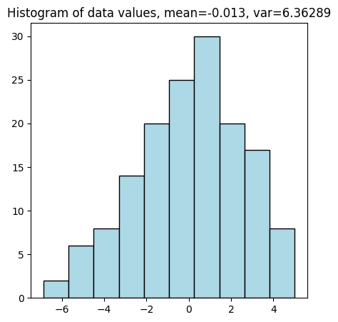
[12]:
# Plot histogram of data values
plt.figure(figsize=(5,5))
plt.hist(v, color='lightblue', edgecolor='black')
plt.title('Histogram of data values, mean={:.2g}, var={:2g}'.format(np.mean(v), np.var(v)))
plt.show()
In the following steps, one assumes that the bi-point statistics is omni-directional (same in any direction), then omni-directional analysis is done.
Omni-directional variogram cloud
The function geone.covModel.variogramCloud1D is used (see jupyter notebook ex_vario_analysis_data1D).
[13]:
h, g, npair = gn.covModel.variogramCloud1D(x, v)

Omni-directional experimental variogram
The function geone.covModel.variogramExp1D is used (see jupyter notebook ex_vario_analysis_data1D).
[14]:
hexp, gexp, cexp = gn.covModel.variogramExp1D(x, v)
# hexp, gexp, cexp = gn.covModel.variogramExp1D(x, v, variogramCloud=(g, h, npair)) # equivalent (x, v not used)

[15]:
hexp, gexp, cexp = gn.covModel.variogramExp1D(x, v, hmax=30, ncla=12)

Omni-directional model fitting
The function geone.covModel.covModel1D_fit is used to fit a covariance model in 1D (class geone.covModel.CovModel1D) (see jupyter notebook ex_vario_analysis_data1D).
[16]:
cov_model_to_optimize = gn.covModel.CovModel1D(
    elem=[('gaussian',    {'w':np.nan, 'r':np.nan}), # elementary contribution
          ('spherical',   {'w':np.nan, 'r':np.nan}), # elementary contribution
          ('exponential', {'w':np.nan, 'r':np.nan}), # elementary contribution
          ('nugget',      {'w':np.nan})              # elementary contribution
         ], name='')

hmax = 30
cov_model_opt, popt = gn.covModel.covModel1D_fit(x, v, cov_model_to_optimize, hmax=hmax,
                                         bounds=([ 0,   0, 0,  0,  0,  0,  0],  # min value for param. to fit
                                                 [20, 30, 20, 30, 30, 30, 20]), # max value for param. to fit
                                         make_plot=False)
plt.figure(figsize=(10,5))
gn.covModel.plot_variogramExp1D(hexp, gexp, cexp, label='vario exp')
cov_model_opt.plot_model(vario=True, hmax=hmax, label='vario opt') # cov. model in 1D
cov_model_ref.plot_model(vario=True, hmax=hmax, label='vario ref') # cov. model in 1D
plt.legend()
plt.show()
cov_model_opt

[16]:
*** CovModel1D object ***
name = ''
number of elementary contribution(s): 4
elementary contribution 0
    type: gaussian
    parameters:
        w = 2.1333804897770787
        r = 9.043448172435706
elementary contribution 1
    type: spherical
    parameters:
        w = 4.508014958345524
        r = 12.134830189552105
elementary contribution 2
    type: exponential
    parameters:
        w = 9.009041749147105e-05
        r = 5.558859353309096
elementary contribution 3
    type: nugget
    parameters:
        w = 7.99529022088765e-08
*****
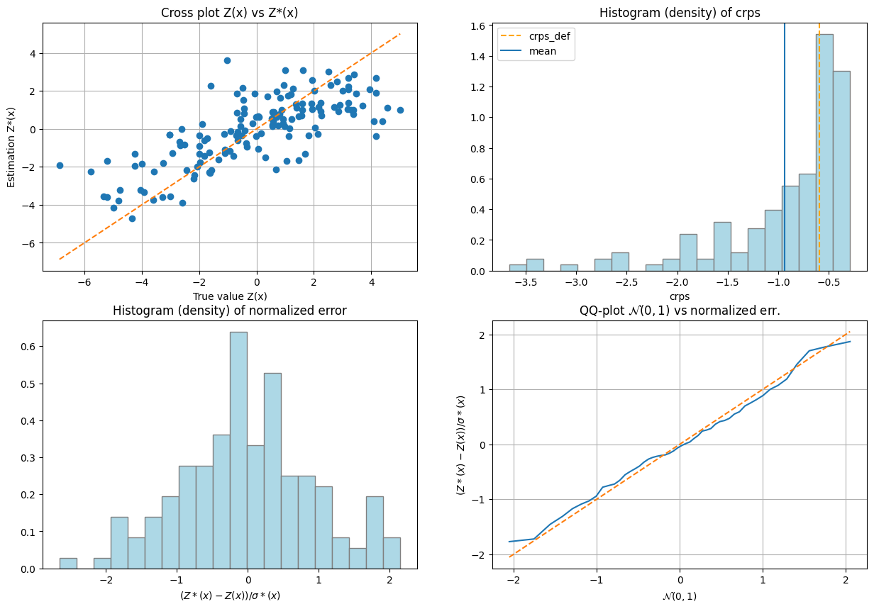
Cross-validation of covariance model by leave-one-out error
The function geone.covModel.cross_valid_loo makes a cross-validation test by leave-one-out (LOO) error.
For a given a data set (in 3D) and a covariance model in 1D, this latter defines an omni-directional covariance model.
See jupyter notebook ex_vario_analysis_data1D for more details about this function.
[17]:
# Interpolation by simple kriging
cv_est1, cv_std1, crps1, crps_def1, pvalue1, success1 = gn.covModel.cross_valid_loo(
                                        x, v, cov_model_opt,
                                        interpolator=gn.covModel.krige,
                                        interpolator_kwargs={'method':'ordinary_kriging'},
                                        print_result=True, make_plot=True, figsize=(15,10), nbins=20)
plt.show()
----- CRPS (negative; the larger, the better) -----
   mean = -0.9358
   def. = -0.5895
----- 1) "Normal law test for mean of normalized error" -----
   p-value = 0.9955
   success = True (wrt significance level 0.05)
      (-> model has no reason to be rejected)
----- 2) "Chi-square test for sum of squares of normalized error" -----
   p-value = 0.8867
   success = True (wrt significance level 0.05)
      (-> model has no reason to be rejected)
----- Statistics of normalized error -----
   mean     = 0.0004619 (should be close to 0)
   std      = 0.9288 (should be close to 1)
   skewness = 0.04562 (should be close to 0)
   excess kurtosis = -0.05457 (should be close to 0)
If one test failed (or if the covariance model does not display the desired shape), the covariance model should be rejected and the search for a convenient covariance model be pursued.
Data interpolation by (simple or ordinary) kriging: function geone.covModel.krige
See notebook ex_vario_analysis_data1D_1.ipynb.
[18]:
# Define points xu where to interpolate
# ... location of the 3D-grid used to build the data set (but it could be different)
xcu = ox + (np.arange(nx)+0.5)*sx # x-coordinates of points
ycu = oy + (np.arange(ny)+0.5)*sy # y-coordinates of points
zcu = oz + (np.arange(nz)+0.5)*sz # z-coordinates of points
zzcu, yycu, xxcu = np.meshgrid(zcu, ycu, xcu, indexing='ij')
xu = np.array((xxcu.reshape(-1), yycu.reshape(-1), zzcu.reshape(-1))).T # 2-dimensional array
# of shape nx*ny*nz x 3
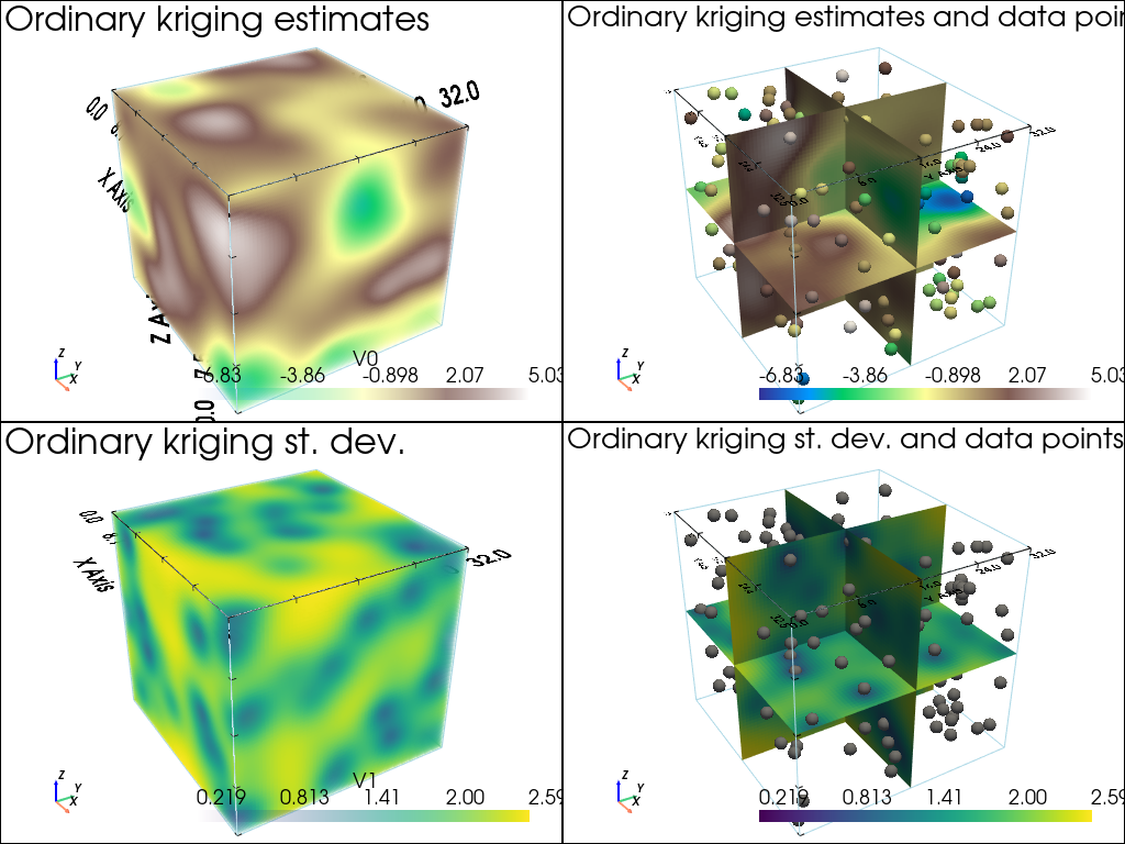
# Ordinary kriging
t1 = time.time() # start time
vu, vu_std = gn.covModel.krige(x, v, xu, cov_model_opt, method='ordinary_kriging', use_unique_neighborhood=True)
# vu: 1-dimensional array, kriging estimates at location xu
# vu_std: 1-dimensional array, kriging standard deviation at location xu
t2 = time.time() # end time
print(f'Elapsed time: {t2-t1:.4g} sec')
# Fill image (Img class from geone.img) for view
# variable 0: kriging estimates
# variable 1: kriging standard deviation
im_krig = gn.img.Img(nx, ny, nz, sx, sy, sz, ox, oy, oz, nv=2, val=np.array((vu, vu_std)))
Elapsed time: 2.308 sec
[19]:
# Color settings
cmap = 'terrain'

cmin = im_krig.vmin()[0] # min value of kriging estimates
cmax = im_krig.vmax()[0] # max value of kriging estimates

# Get colors for conditioning data according to their value and color settings
data_points_col = gn.imgplot.get_colors_from_values(v, cmap=cmap, cmin=cmin, cmax=cmax)

# Set points to be plotted
data_points = pv.PolyData(x)
data_points['colors'] = data_points_col

# Plot "interactive in pop-up window" or "inline" (comment the undesired one) ...
# ... interactive (after closing the pop-up window, the position of the camera is retrieved in output)
#pp = pv.Plotter(shape=(2,2), notebook=False)
# ... inline
pp = pv.Plotter(shape=(2,2))

pp.subplot(0, 0)
gn.imgplot3d.drawImage3D_volume(
    im_krig, iv=0,
    plotter=pp,
    cmap=cmap, cmin=cmin, cmax=cmax,
    show_bounds=True, # show axes and ticks around the 3D box
    text='Ordinary kriging estimates') # title

pp.subplot(0, 1)
gn.imgplot3d.drawImage3D_slice(
    im_krig, iv=0,
    plotter=pp,
    slice_normal_x=ox+(0.5+nx//2)*sx, # near central cell along x
    slice_normal_y=oy+(0.5+ny//2)*sy, # near central cell along y
    slice_normal_z=oz+(0.5+nz//2)*sz, # near central cell along z
    cmap=cmap, cmin=cmin, cmax=cmax,
    show_bounds=True, # show axes and ticks around the 3D box
    scalar_bar_kwargs={'title':''}, # distinct title in each subplot for correct display!
    text='Ordinary kriging estimates and data points') # title
pp.add_mesh(data_points, rgb=True, point_size=12., render_points_as_spheres=True)

pp.subplot(1, 0)
gn.imgplot3d.drawImage3D_volume(
    im_krig, iv=1,
    plotter=pp,
    cmap='viridis',
    show_bounds=True, # show axes and ticks around the 3D box
    text='Ordinary kriging st. dev.') # title

pp.subplot(1, 1)
gn.imgplot3d.drawImage3D_slice(
    im_krig, iv=1,
    plotter=pp,
    slice_normal_x=ox+(0.5+nx//2)*sx, # near central cell along x
    slice_normal_y=oy+(0.5+ny//2)*sy, # near central cell along y
    slice_normal_z=oz+(0.5+nz//2)*sz, # near central cell along z
    cmap='viridis',
    show_bounds=True, # show axes and ticks around the 3D box
    scalar_bar_kwargs={'title':' '}, # distinct title in each subplot for correct display!
    text='Ordinary kriging st. dev. and data points') # title
pp.add_mesh(data_points, color='gray', point_size=12., render_points_as_spheres=True)

pp.link_views()

pp.show(cpos=(165, -100, 115)) # position of the camera can be specified
[20]:
# Define points xu where to interpolate
# ... location of the 3D-grid used to build the data set (but it could be different)
xcu = ox + (np.arange(nx)+0.5)*sx # x-coordinates of points
ycu = oy + (np.arange(ny)+0.5)*sy # y-coordinates of points
zcu = oz + (np.arange(nz)+0.5)*sz # z-coordinates of points
zzcu, yycu, xxcu = np.meshgrid(zcu, ycu, xcu, indexing='ij')
xu = np.array((xxcu.reshape(-1), yycu.reshape(-1), zzcu.reshape(-1))).T # 2-dimensional array
                                                                        # of shape nx*ny*nz x 3

# Simple kriging
t1 = time.time() # start time
vu, vu_std = gn.covModel.krige(x, v, xu, cov_model_opt, method='simple_kriging', use_unique_neighborhood=True)
# vu:     1-dimensional array, kriging estimates at location xu
# vu_std: 1-dimensional array, kriging standard deviation at location xu
t2 = time.time() # end time
print(f'Elapsed time: {t2-t1:.4g} sec')

# Fill image (Img class from geone.img) for view
#   variable 0: kriging estimates
#   variable 1: kriging standard deviation
im_krig = gn.img.Img(nx, ny, nz, sx, sy, sz, ox, oy, oz, nv=2, val=np.array((vu, vu_std)))
Elapsed time: 2.164 sec
[21]:
# Color settings
cmap = 'terrain'

cmin = im_krig.vmin()[0] # min value of kriging estimates
cmax = im_krig.vmax()[0] # max value of kriging estimates

# Get colors for conditioning data according to their value and color settings
data_points_col = gn.imgplot.get_colors_from_values(v, cmap=cmap, cmin=cmin, cmax=cmax)

# Set points to be plotted
data_points = pv.PolyData(x)
data_points['colors'] = data_points_col

# Plot "interactive in pop-up window" or "inline" (comment the undesired one) ...
# ... interactive (after closing the pop-up window, the position of the camera is retrieved in output)
#pp = pv.Plotter(shape=(2,2), notebook=False)
# ... inline
pp = pv.Plotter(shape=(2,2))

pp.subplot(0, 0)
gn.imgplot3d.drawImage3D_volume(
    im_krig, iv=0,
    plotter=pp,
    cmap=cmap, cmin=cmin, cmax=cmax,
    show_bounds=True, # show axes and ticks around the 3D box
    text='Simple kriging estimates') # title

pp.subplot(0, 1)
gn.imgplot3d.drawImage3D_slice(
    im_krig, iv=0,
    plotter=pp,
    slice_normal_x=ox+(0.5+nx//2)*sx, # near central cell along x
    slice_normal_y=oy+(0.5+ny//2)*sy, # near central cell along y
    slice_normal_z=oz+(0.5+nz//2)*sz, # near central cell along z
    cmap=cmap, cmin=cmin, cmax=cmax,
    show_bounds=True, # show axes and ticks around the 3D box
    scalar_bar_kwargs={'title':''}, # distinct title in each subplot for correct display!
    text='Simple kriging estimates and data points') # title
pp.add_mesh(data_points, rgb=True, point_size=12., render_points_as_spheres=True)

pp.subplot(1, 0)
gn.imgplot3d.drawImage3D_volume(
    im_krig, iv=1,
    plotter=pp,
    cmap='viridis',
    show_bounds=True, # show axes and ticks around the 3D box
    text='Simple kriging st. dev.') # title

pp.subplot(1, 1)
gn.imgplot3d.drawImage3D_slice(
    im_krig, iv=1,
    plotter=pp,
    slice_normal_x=ox+(0.5+nx//2)*sx, # near central cell along x
    slice_normal_y=oy+(0.5+ny//2)*sy, # near central cell along y
    slice_normal_z=oz+(0.5+nz//2)*sz, # near central cell along z
    cmap='viridis',
    show_bounds=True, # show axes and ticks around the 3D box
    scalar_bar_kwargs={'title':' '}, # distinct title in each subplot for correct display!
    text='Simple kriging st. dev. and data points') # title
pp.add_mesh(data_points, color='gray', point_size=12., render_points_as_spheres=True)

pp.link_views()

pp.show(cpos=(165, -100, 115)) # position of the camera can be specified

Kriging estimation and simulation in a grid
The function above (gn.covModel.krige and gn.covModel.sgs[_mp]) should not be used for kriging and SGS in a regular grid. Use the dedicated functions (much faster):
geone.geosclassicinterface.estimate: estimation (kriging) in a gridgeone.geosclassicinterface.simulate: simulation (SGS) in a gridgeone.grf.krige<d>D: estimation (kriging) in a<d>-dimensional gridgeone.grf.grf<d>D: simulation (SGS) in a<d>-dimensional grid
Note: the functions of the module ``geone.grf`` are based on “Fast Fourier Transform” and allow for simple kriging only, and do not handle error on data or inequality data.
Note: the function ``geone.multiGaussian.multiGaussianRun`` can be used as a wrapper to run the functions above.
See notebook ex_vario_analysis_data1D_1.ipynb.
Examples
Estimation using the function geone.covModel.krige
[22]:
t1 = time.time()
vu, vu_std = gn.covModel.krige(x, v, xu, cov_model_opt, method='simple_kriging', use_unique_neighborhood=True)
t2 = time.time()
print('Elapsed time: {:.2g} sec'.format(t2-t1))
Elapsed time: 2.1 sec
Estimation using the function geone.grf.krige3D
Via the function geone.multiGaussian.multiGaussianRun, with keyword arguments mode='estimation', algo='fft'.
[23]:
t1 = time.time()
im_grf = gn.multiGaussian.multiGaussianRun(
                cov_model_opt, (nx, ny, nz), (sx, sy, sz), (ox, oy, oz),
                x=x, v=v,
                mode='estimation', algo='fft', output_mode='img')
# # Or:
# vu_grf, vu_std_grf = gn.grf.krige3D(
#                 cov_model_opt, (nx, ny, nz), (sx, sy, sz), (ox, oy, oz),
#                 x=x, v=v)
# im_grf = gn.img.Img(nx, ny, nz, sx, sy, sz, ox, oy, oz, nv=2, val=np.array((vu_grf, vu_std_grf)))
t2 = time.time()
print('Elapsed time: {:.2g} sec'.format(t2-t1))
krige3D: compute circulant embedding...
krige3D: embedding dimension: 128 x 128 x 64
krige3D: compute FFT of circulant matrix...
krige3D: compute covariance matrix (rAA) for conditioning locations...
krige3D: compute covariance matrix (rBA) for non-conditioning / conditioning locations...
krige3D: compute rBA * rAA^(-1)...
krige3D: compute kriging estimates...
krige3D: compute kriging standard deviation ...
Elapsed time: 1.9 sec
Estimation using the function geone.geosclassicinterface.estimate
Via the function geone.multiGaussian.multiGaussianRun, with keyword arguments mode='estimation', algo='classic'.
[24]:
t1 = time.time()
im_gci = gn.multiGaussian.multiGaussianRun(
                cov_model_opt, (nx, ny, nz), (sx, sy, sz), (ox, oy, oz),
                x=x, v=v,
                mode='estimation', algo='classic', output_mode='img',
                method='simple_kriging',
                nneighborMax=24,
                nthreads=8)
# # Or:
# estim_gci = gn.geosclassicinterface.estimate(
#                 cov_model_opt, (nx, ny, nz), (sx, sy, sz), (ox, oy, oz),
#                 x=x, v=v,
#                 method='simple_kriging',
#                 nneighborMax=24,
#                 nthreads=8)
# im_gci = estim_gci['image']
t2 = time.time()
print('Elapsed time: {:.2g} sec'.format(t2-t1))
estimate: pre-process data done: final number of data points : 150, inequality data points: 0
estimate: computational resources: nthreads = 8, nproc_sgs_at_ineq = 8
estimate: (Step 1) no inequality data
estimate: (Step 2) set new dataset gathering data and inequality data locations...
estimate: (Step 3) do kriging at the center of grid cells containing at least one data point...
estimate: (Step 4) do kriging on the grid (at cell centers) using data points at cell centers...
estimate: call `run_MPDSOMPGeosClassicSim` [1 process of 8 thread(s) (OpenMP)] ...
estimate: `run_MPDSOMPGeosClassicSim` [1 process] complete
Elapsed time: 19 sec
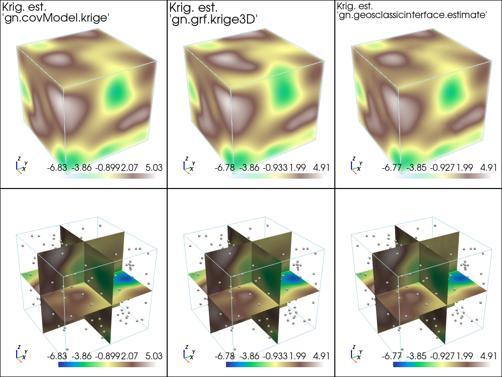
Plot results of estimation
[25]:
# Fill images (Img class from geone.img) for view
#   variable 0: kriging estimates
#   variable 1: kriging standard deviation
im_krig = gn.img.Img(nx, ny, nz, sx, sy, sz, ox, oy, oz, nv=2, val=np.array((vu, vu_std)))
[26]:
# Plot kriging estimates

# Color settings
cmap = 'terrain'

# Plot "interactive in pop-up window" or "inline" (comment the undesired one) ...
# ... interactive (after closing the pop-up window, the position of the camera is retrieved in output)
#pp = pv.Plotter(shape=(2,3), notebook=False)
# ... inline
pp = pv.Plotter(shape=(2,3))

pp.subplot(0, 0)
gn.imgplot3d.drawImage3D_volume(
    im_krig, iv=0,
    plotter=pp,
    cmap=cmap,
    scalar_bar_kwargs={'title':''}, # distinct title in each subplot for correct display!
    text="Krig. est.\n'gn.covModel.krige'", # title
    text_kwargs={'font_size':14}) # font size for title

pp.subplot(0, 1)
gn.imgplot3d.drawImage3D_volume(
    im_grf, iv=0,
    plotter=pp,
    cmap=cmap,
    scalar_bar_kwargs={'title':' '}, # distinct title in each subplot for correct display!
    text="Krig. est.\n'gn.grf.krige3D'", # title
    text_kwargs={'font_size':14}) # font size for title

pp.subplot(0, 2)
gn.imgplot3d.drawImage3D_volume(
    im_gci, iv=0,
    plotter=pp,
    cmap=cmap,
    scalar_bar_kwargs={'title':'  '}, # distinct title in each subplot for correct display!
    text="Krig. est.\n'gn.geosclassicinterface.estimate'", # title
    text_kwargs={'font_size':14}) # font size for title

pp.subplot(1, 0)
gn.imgplot3d.drawImage3D_slice(
    im_krig, iv=0,
    plotter=pp,
    slice_normal_x=ox+(0.5+nx//2)*sx, # near central cell along x
    slice_normal_y=oy+(0.5+ny//2)*sy, # near central cell along y
    slice_normal_z=oz+(0.5+nz//2)*sz, # near central cell along z
    cmap=cmap,
    scalar_bar_kwargs={'title':'   '}, # distinct title in each subplot for correct display!
    text=None) # title
pp.add_mesh(data_points, color=(0.9, 0.9, 0.9), point_size=5., render_points_as_spheres=True)

pp.subplot(1, 1)
gn.imgplot3d.drawImage3D_slice(
    im_grf, iv=0,
    plotter=pp,
    slice_normal_x=ox+(0.5+nx//2)*sx, # near central cell along x
    slice_normal_y=oy+(0.5+ny//2)*sy, # near central cell along y
    slice_normal_z=oz+(0.5+nz//2)*sz, # near central cell along z
    cmap=cmap,
    scalar_bar_kwargs={'title':'    '}, # distinct title in each subplot for correct display!
    text=None) # title
pp.add_mesh(data_points, color=(0.9, 0.9, 0.9), point_size=5., render_points_as_spheres=True)

pp.subplot(1, 2)
gn.imgplot3d.drawImage3D_slice(
    im_gci, iv=0,
    plotter=pp,
    slice_normal_x=ox+(0.5+nx//2)*sx, # near central cell along x
    slice_normal_y=oy+(0.5+ny//2)*sy, # near central cell along y
    slice_normal_z=oz+(0.5+nz//2)*sz, # near central cell along z
    cmap=cmap,
    scalar_bar_kwargs={'title':'     '}, # distinct title in each subplot for correct display!
    text=None) # title
pp.add_mesh(data_points, color=(0.9, 0.9, 0.9), point_size=5., render_points_as_spheres=True)

pp.link_views()

pp.show(cpos=(165, -100, 115)) # position of the camera can be specified
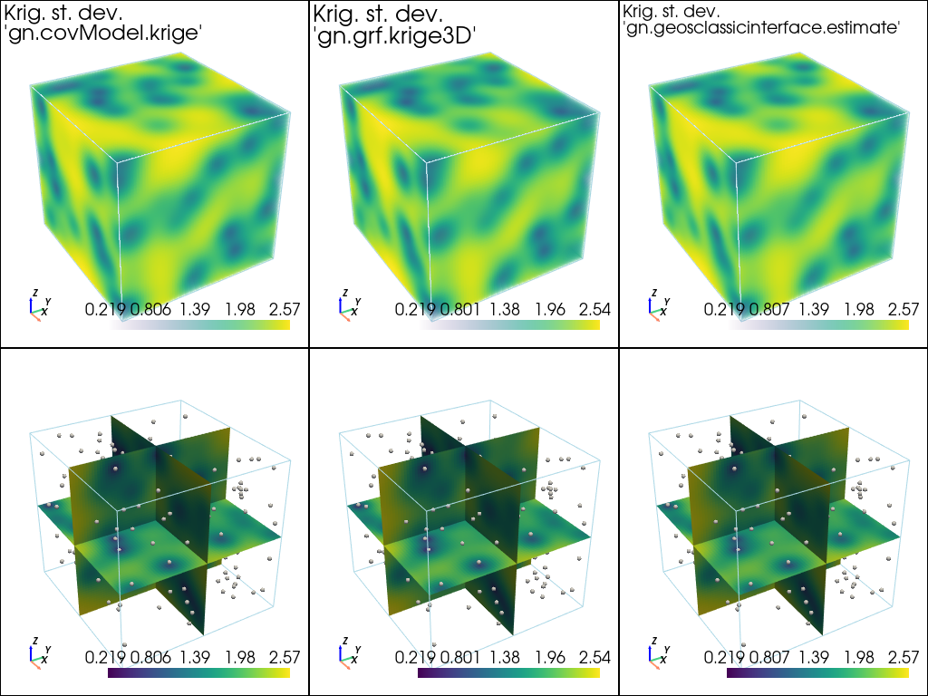
[27]:
# Plot kriging standard deviation

# Plot "interactive in pop-up window" or "inline" (comment the undesired one) ...
# ... interactive (after closing the pop-up window, the position of the camera is retrieved in output)
#pp = pv.Plotter(shape=(2,3), notebook=False)
# ... inline
pp = pv.Plotter(shape=(2,3))

pp.subplot(0, 0)
gn.imgplot3d.drawImage3D_volume(
    im_krig, iv=1,
    plotter=pp,
    cmap='viridis',
    scalar_bar_kwargs={'title':''}, # distinct title in each subplot for correct display!
    text="Krig. st. dev.\n'gn.covModel.krige'", # title
    text_kwargs={'font_size':14}) # font size for title

pp.subplot(0, 1)
gn.imgplot3d.drawImage3D_volume(
    im_grf, iv=1,
    plotter=pp,
    cmap='viridis',
    scalar_bar_kwargs={'title':' '}, # distinct title in each subplot for correct display!
    text="Krig. st. dev.\n'gn.grf.krige3D'", # title
    text_kwargs={'font_size':14}) # font size for title

pp.subplot(0, 2)
gn.imgplot3d.drawImage3D_volume(
    im_gci, iv=1,
    plotter=pp,
    cmap='viridis',
    scalar_bar_kwargs={'title':'  '}, # distinct title in each subplot for correct display!
    text="Krig. st. dev.\n'gn.geosclassicinterface.estimate'", # title
    text_kwargs={'font_size':14}) # font size for title

pp.subplot(1, 0)
gn.imgplot3d.drawImage3D_slice(
    im_krig, iv=1,
    plotter=pp,
    slice_normal_x=ox+(0.5+nx//2)*sx, # near central cell along x
    slice_normal_y=oy+(0.5+ny//2)*sy, # near central cell along y
    slice_normal_z=oz+(0.5+nz//2)*sz, # near central cell along z
    cmap='viridis',
    scalar_bar_kwargs={'title':'   '}, # distinct title in each subplot for correct display!
    text=None) # title
pp.add_mesh(data_points, color=(0.9, 0.9, 0.9), point_size=5., render_points_as_spheres=True)

pp.subplot(1, 1)
gn.imgplot3d.drawImage3D_slice(
    im_grf, iv=1,
    plotter=pp,
    slice_normal_x=ox+(0.5+nx//2)*sx, # near central cell along x
    slice_normal_y=oy+(0.5+ny//2)*sy, # near central cell along y
    slice_normal_z=oz+(0.5+nz//2)*sz, # near central cell along z
    cmap='viridis',
    scalar_bar_kwargs={'title':'    '}, # distinct title in each subplot for correct display!
    text=None) # title
pp.add_mesh(data_points, color=(0.9, 0.9, 0.9), point_size=5., render_points_as_spheres=True)

pp.subplot(1, 2)
gn.imgplot3d.drawImage3D_slice(
    im_gci, iv=1,
    plotter=pp,
    slice_normal_x=ox+(0.5+nx//2)*sx, # near central cell along x
    slice_normal_y=oy+(0.5+ny//2)*sy, # near central cell along y
    slice_normal_z=oz+(0.5+nz//2)*sz, # near central cell along z
    cmap='viridis',
    scalar_bar_kwargs={'title':'     '}, # distinct title in each subplot for correct display!
    text=None) # title
pp.add_mesh(data_points, color=(0.9, 0.9, 0.9), point_size=5., render_points_as_spheres=True)

pp.link_views()

pp.show(cpos=(165, -100, 115)) # position of the camera can be specified
[28]:
print("Peak-to-peak estimation 'gn.covModel.krige - gn.grf.krige3D'                   = {}".format(np.ptp(im_krig.val[0] - im_grf.val[0])))
print("Peak-to-peak estimation 'gn.covModel.krige - gn.geosclassicinterface.estimate' = {}".format(np.ptp(im_krig.val[0] - im_gci.val[0])))
print("Peak-to-peak estimation 'gn.grf.krige3D    - gn.geosclassicinterface.estimate' = {}".format(np.ptp(im_grf.val[0] - im_gci.val[0])))
print("Peak-to-peak st. dev.   'gn.covModel.krige - gn.grf.krige3D'                   = {}".format(np.ptp(im_krig.val[1] - im_grf.val[1])))
print("Peak-to-peak st. dev.   'gn.covModel.krige - gn.geosclassicinterface.estimate' = {}".format(np.ptp(im_krig.val[1] - im_gci.val[1])))
print("Peak-to-peak st. dev.   'gn.grf.krige3D    - gn.geosclassicinterface.estimate' = {}".format(np.ptp(im_grf.val[1] - im_gci.val[1])))
Peak-to-peak estimation 'gn.covModel.krige - gn.grf.krige3D'                   = 3.9329387486203378
Peak-to-peak estimation 'gn.covModel.krige - gn.geosclassicinterface.estimate' = 2.0258586350203265
Peak-to-peak estimation 'gn.grf.krige3D    - gn.geosclassicinterface.estimate' = 4.180550548317362
Peak-to-peak st. dev.   'gn.covModel.krige - gn.grf.krige3D'                   = 0.9922335217643207
Peak-to-peak st. dev.   'gn.covModel.krige - gn.geosclassicinterface.estimate' = 0.4616521097608721
Peak-to-peak st. dev.   'gn.grf.krige3D    - gn.geosclassicinterface.estimate' = 0.7637757109552673
Conditional simulation using the function geone.grf.grf3D
Via the function geone.multiGaussian.multiGaussianRun, with keyword arguments mode='simulation', algo='fft'.
[29]:
np.random.seed(293)

t1 = time.time()
nreal = 20
im_sim_grf = gn.multiGaussian.multiGaussianRun(
                    cov_model_opt, (nx, ny, nz), (sx, sy, sz), (ox, oy, oz),
                    x=x, v=v,
                    mode='simulation', algo='fft', output_mode='img',
                    nreal=nreal)
# # Or:
# sim_grf = gn.grf.grf3D(
#                     cov_model_opt, (nx, ny, nz), (sx, sy, sz), (ox, oy, oz),
#                     x=x, v=v,
#                     nreal=nreal)
# im_sim_grf = gn.img.Img(nx, ny, nz, sx, sy, sz, ox, oy, oz, nv=nreal, val=sim_grf)
t2 = time.time()
print('Elapsed time: {:.2g} sec'.format(t2-t1))
grf3D: do preliminary computation...
grf3D: compute circulant embedding...
grf3D: embedding dimension: 128 x 128 x 64
grf3D: compute FFT of circulant matrix...
grf3D: treatment of conditioning data...
grf3D: compute covariance matrix (rAA) for conditioning locations...
grf3D: compute index in the embedding grid for non-conditioning / conditioning locations...
Elapsed time: 3.4 sec
Conditional simulation using the function geone.geosclassicinterface.simulate
Via the function geone.multiGaussian.multiGaussianRun, with keyword arguments mode='simulation', algo='classic', and specifying the computational resources (nproc and nthreads_per_proc).
[30]:
np.random.seed(293)

t1 = time.time()
nreal = 20
im_sim_gci = gn.multiGaussian.multiGaussianRun(
                    cov_model_opt, (nx, ny, nz), (sx, sy, sz), (ox, oy, oz),
                    x=x, v=v,
                    mode='simulation', algo='classic', output_mode='img',
                    method='simple_kriging',
                    nreal=nreal,
                    nproc=2, nthreads_per_proc=4)
# # Or:
# sim_gci = gn.geosclassicinterface.simulate(
#                     cov_model_opt, (nx, ny, nz), (sx, sy, sz), (ox, oy, oz),
#                     x=x, v=v,
#                     method='simple_kriging',
#                     nreal=nreal,
#                     nproc=4, nthreads_per_proc=4)
# im_sim_gci = sim_gci['image']
t2 = time.time()
print('Elapsed time: {:.2g} sec'.format(t2-t1))
simulate: pre-process data done: final number of data points : 150, inequality data points: 0
simulate: computational resources: nproc = 2, nthreads_per_proc = 4, nproc_sgs_at_ineq = 8
simulate: (Step 1) no inequality data
simulate: (Step 2) set new dataset gathering data and inequality data locations...
simulate: (Step 3) do kriging at the center of grid cells containing at least one data point...
simulate: (Step 4) do sgs (20 realizations) on the grid (at cell centers) using data points at cell centers...
simulate: call `run_MPDSOMPGeosClassicSim` [2 process(es) of 4 thread(s) (OpenMP)] ...
simulate: `run_MPDSOMPGeosClassicSim` [2 process(es)] complete
Elapsed time: 6.9 sec
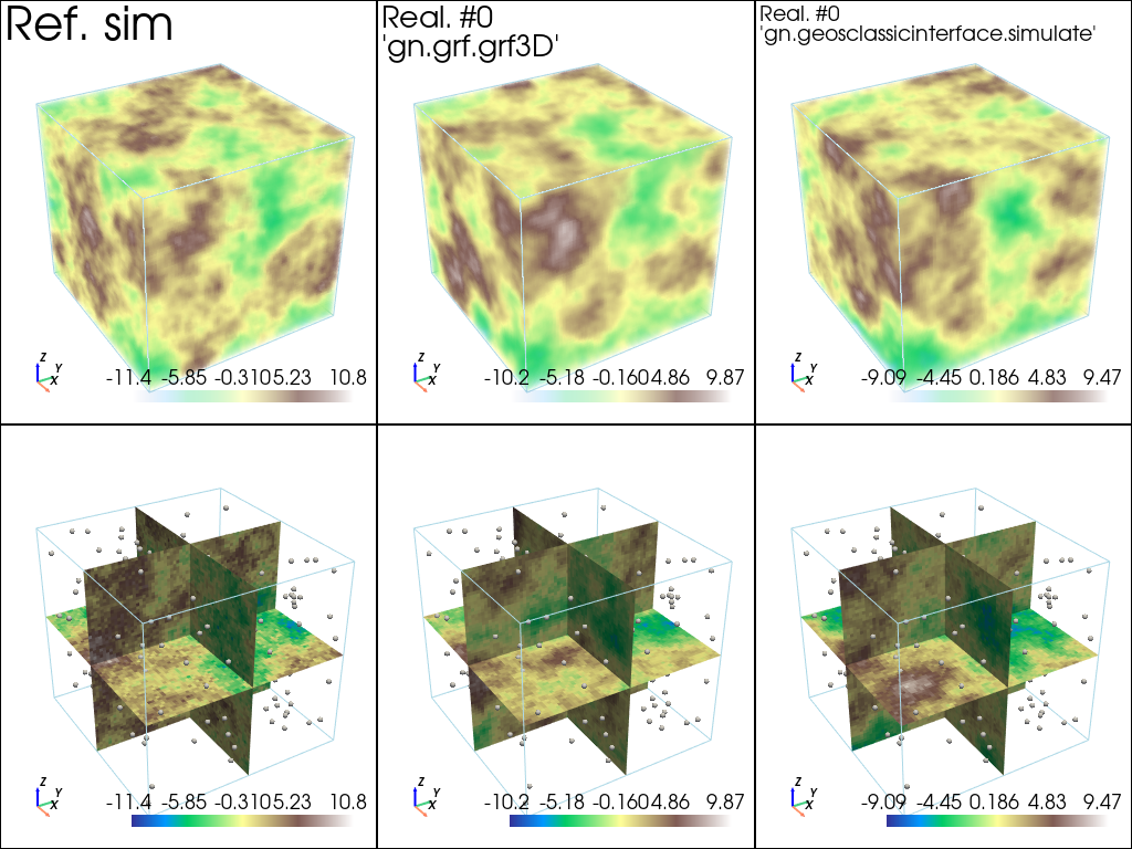
Plot some realizations and compare to the reference simulation
[31]:
# min and max over all real and ref. sim
im_vmin = min(np.min(im_sim_grf.vmin()), np.min(im_sim_gci.vmin()), im_ref.vmin()[0])
im_vmax = max(np.max(im_sim_grf.vmax()), np.min(im_sim_gci.vmax()), im_ref.vmax()[0])
[32]:
# Color settings
cmap = 'terrain'

# Plot "interactive in pop-up window" or "inline" (comment the undesired one) ...
# ... interactive (after closing the pop-up window, the position of the camera is retrieved in output)
#pp = pv.Plotter(shape=(2,3), notebook=False)
# ... inline
pp = pv.Plotter(shape=(2,3))

pp.subplot(0, 0)
gn.imgplot3d.drawImage3D_volume(
    im_ref, iv=0,
    plotter=pp,
    cmap=cmap,
    scalar_bar_kwargs={'title':''}, # distinct title in each subplot for correct display!
    text="Ref. sim") # title

pp.subplot(0, 1)
gn.imgplot3d.drawImage3D_volume(
    im_sim_grf, iv=0,
    plotter=pp,
    cmap=cmap,
    scalar_bar_kwargs={'title':' '}, # distinct title in each subplot for correct display!
    text="Real. #0\n'gn.grf.grf3D'", # title
    text_kwargs={'font_size':14}) # font size for title

pp.subplot(0, 2)
gn.imgplot3d.drawImage3D_volume(
    im_sim_gci, iv=0,
    plotter=pp,
    cmap=cmap,
    scalar_bar_kwargs={'title':'  '}, # distinct title in each subplot for correct display!
    text="Real. #0\n'gn.geosclassicinterface.simulate'", # title
    text_kwargs={'font_size':14}) # font size for title

pp.subplot(1, 0)
gn.imgplot3d.drawImage3D_slice(
    im_ref, iv=0,
    plotter=pp,
    slice_normal_x=ox+(0.5+nx//2)*sx, # near central cell along x
    slice_normal_y=oy+(0.5+ny//2)*sy, # near central cell along y
    slice_normal_z=oz+(0.5+nz//2)*sz, # near central cell along z
    cmap=cmap,
    scalar_bar_kwargs={'title':'   '}, # distinct title in each subplot for correct display!
    text=None) # title
pp.add_mesh(data_points, color=(0.9, 0.9, 0.9), point_size=5., render_points_as_spheres=True)

pp.subplot(1, 1)
gn.imgplot3d.drawImage3D_slice(
    im_sim_grf, iv=0,
    plotter=pp,
    slice_normal_x=ox+(0.5+nx//2)*sx, # near central cell along x
    slice_normal_y=oy+(0.5+ny//2)*sy, # near central cell along y
    slice_normal_z=oz+(0.5+nz//2)*sz, # near central cell along z
    cmap=cmap,
    scalar_bar_kwargs={'title':'    '}, # distinct title in each subplot for correct display!
    text=None) # title
pp.add_mesh(data_points, color=(0.9, 0.9, 0.9), point_size=5., render_points_as_spheres=True)

pp.subplot(1, 2)
gn.imgplot3d.drawImage3D_slice(
    im_sim_gci, iv=0,
    plotter=pp,
    slice_normal_x=ox+(0.5+nx//2)*sx, # near central cell along x
    slice_normal_y=oy+(0.5+ny//2)*sy, # near central cell along y
    slice_normal_z=oz+(0.5+nz//2)*sz, # near central cell along z
    cmap=cmap,
    scalar_bar_kwargs={'title':'     '}, # distinct title in each subplot for correct display!
    text=None) # title
pp.add_mesh(data_points, color=(0.9, 0.9, 0.9), point_size=5., render_points_as_spheres=True)

pp.link_views()

pp.show(cpos=(165, -100, 115)) # position of the camera can be specified