GEONE - Variogram analysis and kriging for data in 1D with non-stationarity
The goal is to interpolate a non-stationary data set in 1D (based on simple or ordinary kriging) in a domain (grid), where non-stationarity are given as:
local factor (multiplier) for the ranges along the main axes of the covariance model
local factor (multiplier) for the total weight (variance, sill) of the covariance model
One or several of these non-stationary features can be considered.
Import what is required
[1]:
import numpy as np
import matplotlib.pyplot as plt
import time

# import package 'geone'
import geone as gn
[2]:
# Show version of python and version of geone
import sys
print(sys.version_info)
print('geone version: ' + gn.__version__)
sys.version_info(major=3, minor=13, micro=7, releaselevel='final', serial=0)
geone version: 1.3.1
Remark
The matplotlib figures can be visualized in interactive mode:
%matplotlib notebook: enable interactive mode%matplotlib inline: disable interactive mode
I. Build non-stationary features on a grid
Here are built the following non-stationary features on a grid:
r_factor_loc: local factor (multiplier) for the range of the covariance modelw_factor_loc: local factor (multiplier) for the total weight (variance, sill) of the covariance model
Defining domain of simulation (grid)
[3]:
nx = 2000 # number of cells
sx = 0.5  # cell unit
ox = 0.0  # origin

xmin, xmax = ox, ox+nx*sx

# # Set an image with simulation grid geometry defined above, and no variable
# im = gn.img.Img(nx, ny, 1, sx, sy, 1., ox, oy, 0., nv=0)
Defining non-stationarities
Range
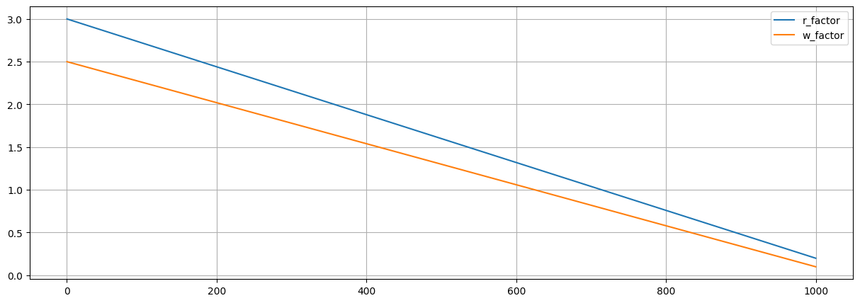
The factor (multiplier) for range r_factor locally varying in the grid is defined as im_r_factor: an image (with one variable on the grid).
Variance (sill)
The factor (multiplier) for the total weight (variance, sill) w_factor locally varying in the grid is defined as im_w_factor: an image (with one variable on the grid).
[4]:
# Define r_factor as r0 on the left of the grid and decreasing linearly when going to the right of the grid
# ---------------
r0 = 3.0 # on the left
r1 = 0.2 # minimal value

# "Empty" image
im_r_factor = gn.img.Img(nx, 1, 1, sx, 1., 1., ox, 0., 0., nv=0)

# Add variable
r = r0 + im_r_factor.x()/im_r_factor.x().max() * (r1-r0)
im_r_factor.append_var(r)

# Define w_factor as w0 on the left of the grid and decreasing linearly when going to the right of the grid
# ---------------
w0 = 2.5 # on the left
w1 = 0.1 # minimal value

# "Empty" image
im_w_factor = gn.img.Img(nx, 1, 1, sx, 1., 1., ox, 0., 0., nv=0)

# Add variable
w = w0 + im_w_factor.xx()/im_w_factor.xx().max() * (w1-w0)
im_w_factor.append_var(w)

# Plot
# ----
plt.figure(figsize=(15,5))
plt.plot(im_r_factor.x(), im_r_factor.val[0,0,0], label='r_factor')
plt.plot(im_w_factor.x(), im_w_factor.val[0,0,0], label='w_factor')
plt.legend()
plt.grid()
plt.show()
II Non-stationary simulations
First define a reference covariance model and generate an unconditional simulation (reference). Then build a data set by extract some points from the simulation. Then, ignoring the covariance model and starting from the data set and the maps controlling the non-stationary features:
fit a covariance model
do kriging / conditional simulations
Several cases are proposed below with different non-stationary features.
A. Non-stationary range
Reference covariance model and non-stationarity
Define first a stationary reference covariance model in 1D. Then, add the desired non-stationarity feature.
[5]:
# Define a base covariance model (stationary)
cov_model_base = gn.covModel.CovModel1D(elem=[
    ('cubic', {'w':10, 'r':50.0}), # elementary contribution
    ], name='ref')

# Set list to handle non-stationarities
cov_model_non_stationarity_list = [
    ('multiply_r', im_r_factor.val[0]), # multiply range by `im_r_factor.val[0]` over the grid
]
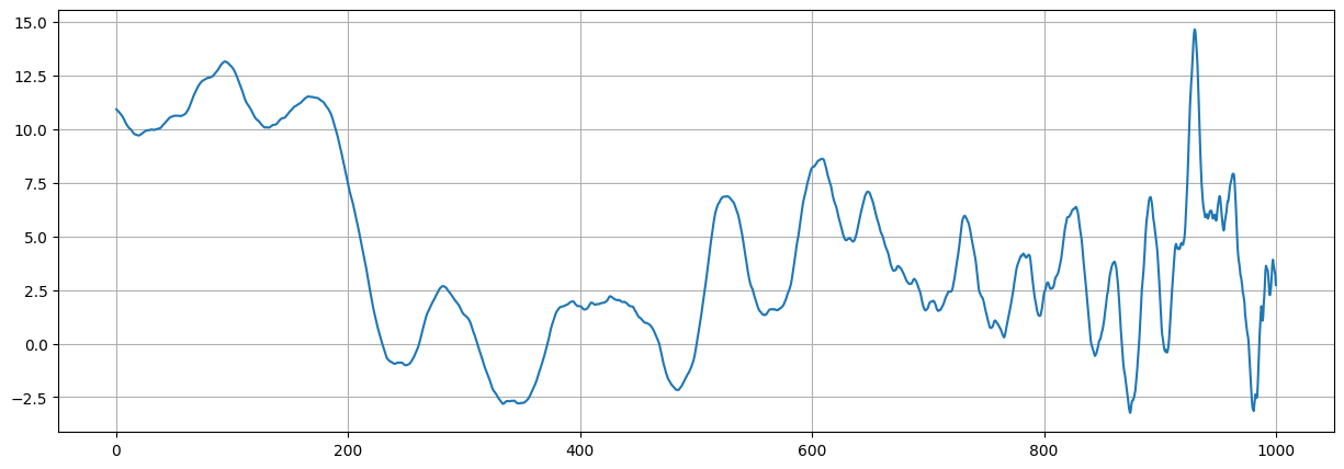
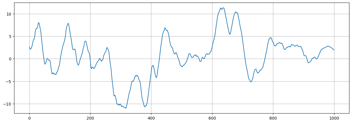
Do an unconditional simulation (reference)
[6]:
# Simulation
nreal = 1
np.random.seed(2385)
geosclassic_output = gn.geosclassicinterface.simulate(
                        cov_model_base, nx, sx, ox,
                        method='ordinary_kriging',
                        cov_model_non_stationarity_list=cov_model_non_stationarity_list,
                        nneighborMax=64,
                        nreal=nreal,
                        nproc=1, nthreads_per_proc=8)

im_ref = geosclassic_output['image']

plt.figure(figsize=(15,5))
plt.plot(im_ref.x(), im_ref.val[0,0,0])
plt.grid()
plt.show()
simulate: pre-process data done: final number of data points : 0, inequality data points: 0
simulate: computational resources: nproc = 1, nthreads_per_proc = 8, nproc_sgs_at_ineq = 8
simulate: (Step 1-3 skipped) no data
simulate: (Step 4) do sgs (1 realizations) on the grid (at cell centers) using data points at cell centers...
simulate: call `run_MPDSOMPGeosClassicSim` [1 process of 8 thread(s) (OpenMP)] ...
simulate: `run_MPDSOMPGeosClassicSim` [1 process] complete
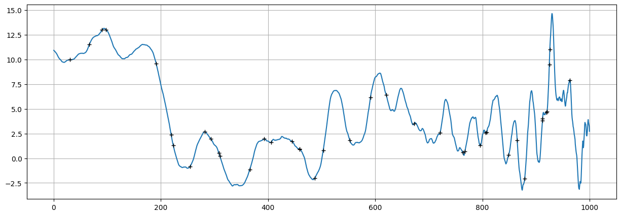
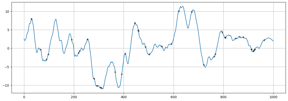
Build a non-stationary data set (1D)
The data set is defined by extracting some points from the simulation of reference.
Note: the data set should contain enough points to catch the non-stationarities.
[7]:
# Extract som points from the simulation
n = 40

# --- Choose 1. or 2. below ---
# # 1. Sampling the image
# ps = gn.img.sampleFromImage(im_ref, n, seed=234)
# # Data points and data value
# x = ps.x()
# v = ps.val[3]
# # Optionally: move points in the grid cells randomly, and add noise to values
# x = x + (np.random.random(n)-0.5)* im_ref.sx
# v = v + (np.random.random(n)-0.5)* 1.e-1

# 2. Using the function interpolating the image values
f = gn.img.Img_interp_func(im_ref, iy=0, iz=0)
np.random.seed(987)
x = im_ref.xmin() + np.random.random(n) * (im_ref.xmax()-im_ref.xmin())
v = f(x)
# ----- #

plt.figure(figsize=(15,5))
plt.plot(im_ref.x(), im_ref.val[0,0,0])
plt.plot(x, v, '+', c='k')
plt.grid()
plt.show()
Simulation starting from a non-stationary data set in 1D and assuming “non-stationarity feature(s)” known
n: number of data pointsx: location of data points (1-dimensional array of lengthn)v: values at data points (1-dimensional array of lengthn)im_r_factor: image of the factor (multiplier)r_factorin the grid; the functionr_factor_inv_loc_func(interpolator of the inverse ofr_factorin the grid) is built from this image
[8]:
# Set a function interpolating the inverse of the r_factor (given location)
im_tmp = gn.img.copyImg(im_r_factor)
im_tmp.val = 1.0/im_tmp.val
r_factor_inv_loc_func = gn.img.Img_interp_func(im_tmp, ind=0, iy=0, iz=0)
# -> specify iy=0, iz=0: consider only x coordinates along the "line" iy=0 and iz=0
Fitting covariance model accounting for non-stationarity
[9]:
cov_model_to_optimize = gn.covModel.CovModel1D(elem=[
        ('cubic', {'w':np.nan, 'r':np.nan}), # elementary contribution
         ], name='')

t1 = time.time()
cov_model_opt, popt = gn.covModel.covModel1D_fit(
                x, v, cov_model_to_optimize,
                coord_factor_loc_func=r_factor_inv_loc_func, # deal with non-stationarity (multiplier for range)
                loc_m=10, # loc_m > 0: number of sub-intervals btw pair of points to estimate local factor (default 1)
                          # loc_m = 0: take factor from one point
                bounds=([   0,   0],  # min value for param. to fit
                        [ 100, 500]), # max value for param. to fit
                hmax=100, make_plot=False) # figure size for plot
t2 = time.time()
print(f'Fitting covariance model - elapsed time: {t2-t1:.4g}')

cov_model_opt
Fitting covariance model - elapsed time: 0.008378
[9]:
*** CovModel1D object ***
name = ''
number of elementary contribution(s): 1
elementary contribution 0
    type: cubic
    parameters:
        w = 26.219740235828276
        r = 144.1487904701664
*****
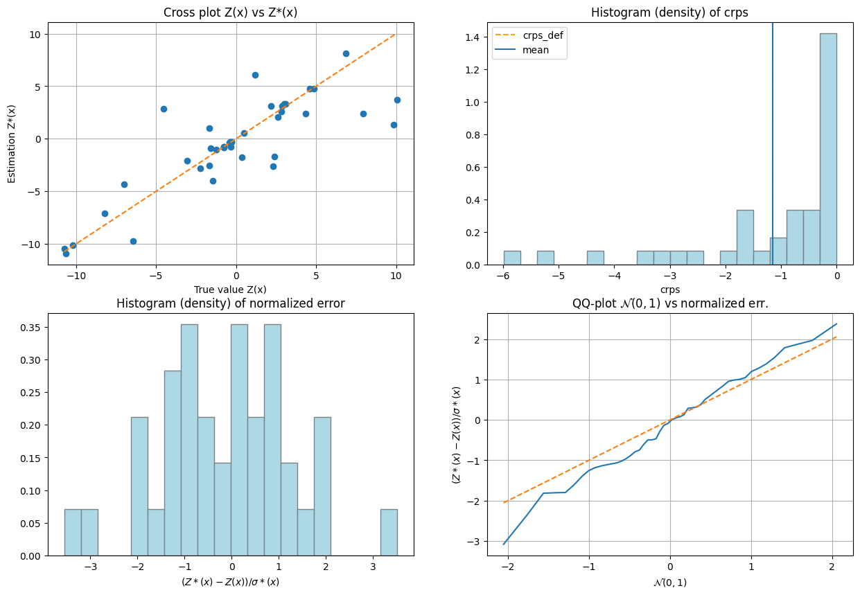
Cross-validation of covariance model by leave-one-out error
The function geone.covModel.cross_valid_loo performs a cross-validation test by leave-one-out (LOO) error.
See jupyter notebook ex_vario_analysis_data1D for more details about this function.
[10]:
# Set a function interpolating the r_factor (given location)
r_factor_loc_func = gn.img.Img_interp_func(im_r_factor, ind=0, iy=0, iz=0)
# -> specify iy=0, iz=0: consider only x coordinates along the "line" iy=0 and iz=0
# Set list to handle non-stationarities at x
cov_model_non_stationarity_x_list = [
('multiply_r', r_factor_loc_func(x))
]
cv_est1, cv_std1, crps1, crps_def1, pvalue1, success1 = gn.covModel.cross_valid_loo(
x, v, cov_model_opt,
interpolator=gn.covModel.krige,
interpolator_kwargs={'method':'ordinary_kriging'},
cov_model_non_stationarity_x_list=cov_model_non_stationarity_x_list,
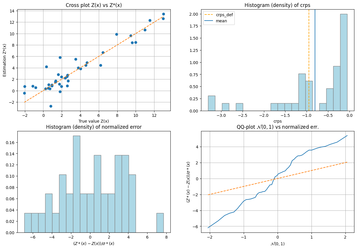
print_result=True, make_plot=True, figsize=(15,10), nbins=20)
plt.show()
----- CRPS (negative; the larger, the better) -----
   mean = -0.8029
   def. = -0.9435
----- 1) "Normal law test for mean of normalized error" -----
   p-value = 0.3073
   success = True (wrt significance level 0.05)
      (-> model has no reason to be rejected)
----- 2) "Chi-square test for sum of squares of normalized error" -----
   p-value = 0
   success = False (wrt significance level 0.05)
      -> model should be REJECTED
----- Statistics of normalized error -----
   mean     = 0.1614 (should be close to 0)
   std      = 3.273 (should be close to 1)
   skewness = -0.08016 (should be close to 0)
   excess kurtosis = -0.6062 (should be close to 0)
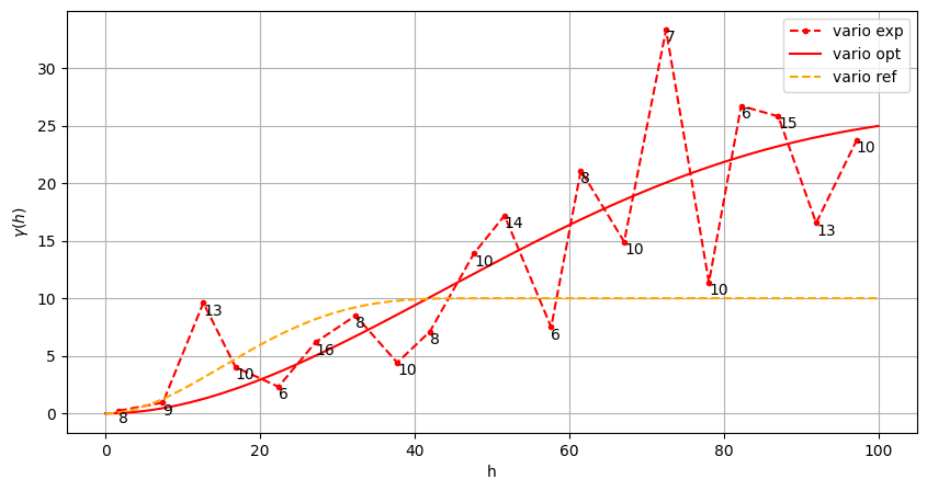
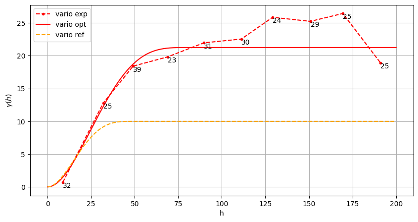
Show experimental variogram, fitted model and reference model
[11]:
hmax = 100.0

hexp, gexp, cexp = gn.covModel.variogramExp1D(x, v, hmax=hmax,
                                              coord_factor_loc_func=r_factor_inv_loc_func, loc_m=10,
                                              ncla=20, make_plot=False)

plt.figure(figsize=(10,5))
gn.covModel.plot_variogramExp1D(hexp, gexp, cexp, c='red', label='vario exp')
cov_model_opt.plot_model(vario=True, hmax=hmax, c='red', label='vario opt')
cov_model_base.plot_model(vario=True, hmax=hmax, c='orange', ls='dashed', label='vario ref')
plt.legend()

plt.show()
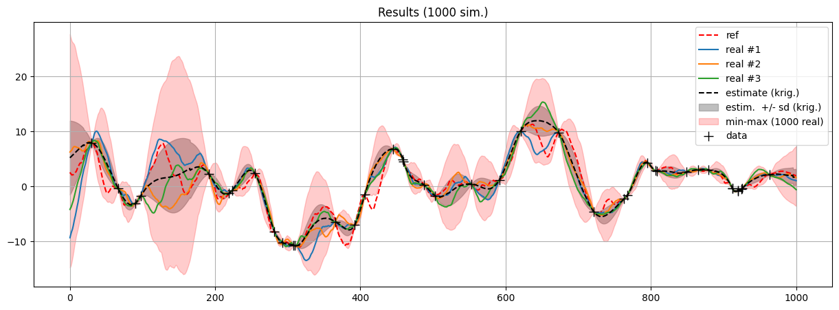
Kriging and conditional simulations
[12]:
# Kriging
t1 = time.time() # start time
geosclassic_output = gn.geosclassicinterface.estimate(
                        cov_model_opt, nx, sx, ox,
                        x=x, v=v,
                        method='ordinary_kriging',
                        cov_model_non_stationarity_list=cov_model_non_stationarity_list,
                        nneighborMax=20,
                        nthreads=8)
t2 = time.time() # end time
print(f'Kriging - elapsed time: {t2-t1:.4g} sec')

# Retrieve kriging estimate and standard deviation
im_krig = geosclassic_output['image']
estimate: pre-process data done: final number of data points : 40, inequality data points: 0
estimate: computational resources: nthreads = 8, nproc_sgs_at_ineq = 8
estimate: (Step 1) no inequality data
estimate: (Step 2) set new dataset gathering data and inequality data locations...
estimate: (Step 3) do kriging at the center of grid cells containing at least one data point...
estimate: (Step 4) do kriging on the grid (at cell centers) using data points at cell centers...
estimate: call `run_MPDSOMPGeosClassicSim` [1 process of 8 thread(s) (OpenMP)] ...
estimate: `run_MPDSOMPGeosClassicSim` [1 process] complete
Kriging - elapsed time: 0.02475 sec
[13]:
# Simulation
nreal = 1000
np.random.seed(22131)
t1 = time.time() # start time
geosclassic_output = gn.geosclassicinterface.simulate(
                        cov_model_opt, nx, sx, ox,
                        x=x, v=v, method='ordinary_kriging',
                        cov_model_non_stationarity_list=cov_model_non_stationarity_list,
                        nneighborMax=20,
                        nreal=nreal,
                        nproc=4, nthreads_per_proc=4)
t2 = time.time() # end time
print(f'{nreal} simul. - elapsed time: {t2-t1:.4g} sec')

# Retrieve the realizations
simul = geosclassic_output['image']

# Compute mean and standard deviation (pixel-wise)
simul_mean = gn.img.imageContStat(simul, op='mean')
simul_std = gn.img.imageContStat(simul, op='std')
simulate: pre-process data done: final number of data points : 40, inequality data points: 0
simulate: computational resources: nproc = 4, nthreads_per_proc = 4, nproc_sgs_at_ineq = 16
simulate: (Step 1) no inequality data
simulate: (Step 2) set new dataset gathering data and inequality data locations...
simulate: (Step 3) do kriging at the center of grid cells containing at least one data point...
simulate: (Step 4) do sgs (1000 realizations) on the grid (at cell centers) using data points at cell centers...
simulate: call `run_MPDSOMPGeosClassicSim` [4 process(es) of 4 thread(s) (OpenMP)] ...
simulate: `run_MPDSOMPGeosClassicSim` [4 process(es)] complete
1000 simul. - elapsed time: 4.33 sec
[14]:
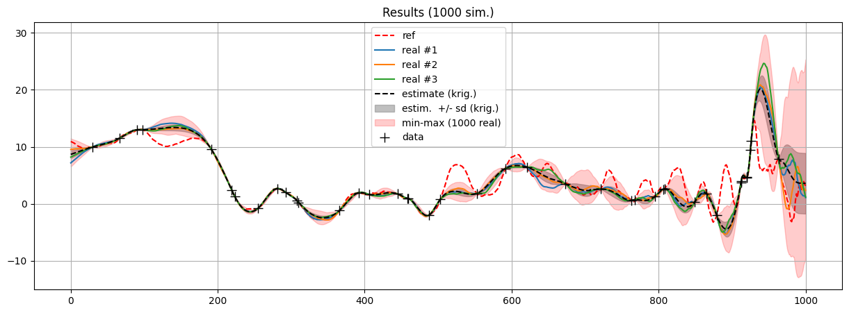
# Plot the first simulations and the results of estimation
plt.figure(figsize=(15,5))

plt.plot(im_ref.x(), im_ref.val[0,0,0,:], c='red', ls='dashed', label='ref')

for i in range(3):
    plt.plot(simul.x(), simul.val[i,0,0,:], label='real #{}'.format(i+1))

plt.plot(im_krig.x(), im_krig.val[0,0,0,:], c='black', ls='dashed', label='estimate (krig.)')
plt.fill_between(im_krig.x(),
                 im_krig.val[0,0,0,:] - im_krig.val[1,0,0,:],
                 im_krig.val[0,0,0,:] + im_krig.val[1,0,0,:],
                 color='gray', alpha=.5, label='estim.  +/- sd (krig.)')

plt.fill_between(simul.x(), simul.val[:,0,0,:].min(axis=0), simul.val[:,0,0,:].max(axis=0),
                 color='red', alpha=.2, label='min-max ({} real)'.format(nreal))

plt.plot(x, v, '+', c='k', markersize=10, label='data') # add conditioning points

plt.grid()
plt.legend()
plt.title(f'Results ({nreal} sim.)')
plt.show()
B. Non-stationary variance (sill)
Reference covariance model and non-stationarity
Define first a stationary reference covariance model in 1D. Then, add the desired non-stationarity feature.
[15]:
# Define a base covariance model (stationary)
cov_model_base = gn.covModel.CovModel1D(elem=[
    ('cubic', {'w':10, 'r':50.0}), # elementary contribution
    ], name='ref')

# Set list to handle non-stationarities
cov_model_non_stationarity_list = [
    ('multiply_w', im_w_factor.val[0]), # multiply weight by `im_w_factor.val[0]` over the grid
]
Do an unconditional simulation (reference)
[16]:
# Simulation
nreal = 1
np.random.seed(2485)
geosclassic_output = gn.geosclassicinterface.simulate(
                        cov_model_base, nx, sx, ox,
                        method='ordinary_kriging',
                        cov_model_non_stationarity_list=cov_model_non_stationarity_list,
                        nneighborMax=64,
                        nreal=nreal,
                        nproc=1, nthreads_per_proc=8)

im_ref = geosclassic_output['image']

plt.figure(figsize=(15,5))
plt.plot(im_ref.x(), im_ref.val[0,0,0])
plt.grid()
plt.show()
simulate: pre-process data done: final number of data points : 0, inequality data points: 0
simulate: computational resources: nproc = 1, nthreads_per_proc = 8, nproc_sgs_at_ineq = 8
simulate: (Step 1-3 skipped) no data
simulate: (Step 4) do sgs (1 realizations) on the grid (at cell centers) using data points at cell centers...
simulate: call `run_MPDSOMPGeosClassicSim` [1 process of 8 thread(s) (OpenMP)] ...
simulate: `run_MPDSOMPGeosClassicSim` [1 process] complete
Build a non-stationary data set (1D)
The data set is defined by extracting some points from the simulation of reference.
Note: the data set should contain enough points to catch the non-stationarities.
[17]:
# Extract som points from the simulation
n = 40

# --- Choose 1. or 2. below ---
# # 1. Sampling the image
# ps = gn.img.sampleFromImage(im_ref, n, seed=234)
# # Data points and data value
# x = ps.x()
# v = ps.val[3]
# # Optionally: move points in the grid cells randomly, and add noise to values
# x = x + (np.random.random(n)-0.5)* im_ref.sx
# v = v + (np.random.random(n)-0.5)* 1.e-1

# 2. Using the function interpolating the image values
f = gn.img.Img_interp_func(im_ref, iy=0, iz=0)
np.random.seed(987)
x = im_ref.xmin() + np.random.random(n) * (im_ref.xmax()-im_ref.xmin())
v = f(x)
# ----- #

plt.figure(figsize=(15,5))
plt.plot(im_ref.x(), im_ref.val[0,0,0])
plt.plot(x, v, '+', c='k')
plt.grid()
plt.show()
Simulation starting from a non-stationary data set in 1D and assuming “non-stationarity feature(s)” known
n: number of data pointsx: location of data points (1-dimensional array of lengthn)v: values at data points (1-dimensional array of lengthn)im_w_factor: image of the factor (multiplier)w_factorin the grid; the functionw_factor_inv_loc_func(interpolator of the inverse ofw_factorin the grid) is built from this image
[18]:
# Set a function interpolating the inverse of the w_factor (given location)
im_tmp = gn.img.copyImg(im_w_factor)
im_tmp.val = 1.0/im_tmp.val
w_factor_inv_loc_func = gn.img.Img_interp_func(im_tmp, ind=0, iy=0, iz=0)
# -> specify iy=0, iz=0: consider only x coordinates along the "line" iy=0 and iz=0
Fitting covariance model accounting for non-stationarity
[19]:
cov_model_to_optimize = gn.covModel.CovModel1D(elem=[
        ('cubic', {'w':np.nan, 'r':np.nan}), # elementary contribution
         ], name='')

t1 = time.time()
cov_model_opt, popt = gn.covModel.covModel1D_fit(
                x, v, cov_model_to_optimize,
                w_factor_loc_func=w_factor_inv_loc_func, # deal with non-stationarity (multiplier for weight)
                loc_m=10, # loc_m > 0: number of sub-intervals btw pair of points to estimate local factor (default 1)
                          # loc_m = 0: take factor from one point
                bounds=([   0,   0],  # min value for param. to fit
                        [ 100, 500]), # max value for param. to fit
                hmax=100, make_plot=False) # figure size for plot
t2 = time.time()
print(f'Fitting covariance model - elapsed time: {t2-t1:.4g}')

cov_model_opt
Fitting covariance model - elapsed time: 0.00691
[19]:
*** CovModel1D object ***
name = ''
number of elementary contribution(s): 1
elementary contribution 0
    type: cubic
    parameters:
        w = 21.250098976072714
        r = 81.84710526696728
*****
Cross-validation of covariance model by leave-one-out error
The function geone.covModel.cross_valid_loo performs a cross-validation test by leave-one-out (LOO) error.
See jupyter notebook ex_vario_analysis_data1D for more details about this function.
[20]:
# Set a function interpolating the w_factor (given location)
w_factor_loc_func = gn.img.Img_interp_func(im_w_factor, ind=0, iy=0, iz=0)
# -> specify iy=0, iz=0: consider only x coordinates along the "line" iy=0 and iz=0

# Set list to handle non-stationarities at x
cov_model_non_stationarity_x_list = [
    ('multiply_w', w_factor_loc_func(x))
]

cv_est1, cv_std1, crps1, crps_def1, pvalue1, success1 = gn.covModel.cross_valid_loo(
                                        x, v, cov_model_opt,
                                        interpolator=gn.covModel.krige,
                                        interpolator_kwargs={'method':'ordinary_kriging'},
                                        cov_model_non_stationarity_x_list=cov_model_non_stationarity_x_list,
                                        print_result=True, make_plot=True, figsize=(15,10), nbins=20)
plt.show()
----- CRPS (negative; the larger, the better) -----
   mean = -1.149
   def. = -1.151
----- 1) "Normal law test for mean of normalized error" -----
   p-value = 0.504
   success = True (wrt significance level 0.05)
      (-> model has no reason to be rejected)
----- 2) "Chi-square test for sum of squares of normalized error" -----
   p-value = 0.0003299
   success = False (wrt significance level 0.05)
      -> model should be REJECTED
----- Statistics of normalized error -----
   mean     = -0.1057 (should be close to 0)
   std      = 1.389 (should be close to 1)
   skewness = -0.0118 (should be close to 0)
   excess kurtosis = 0.2549 (should be close to 0)
Show experimental variogram, fitted model and reference model
[21]:
hmax = 200.0

hexp, gexp, cexp = gn.covModel.variogramExp1D(x, v, hmax=hmax,
                                              w_factor_loc_func=w_factor_inv_loc_func, loc_m=10,
                                              ncla=10, make_plot=False)

plt.figure(figsize=(10,5))
gn.covModel.plot_variogramExp1D(hexp, gexp, cexp, c='red', label='vario exp')
cov_model_opt.plot_model(vario=True, hmax=hmax, c='red', label='vario opt')
cov_model_base.plot_model(vario=True, hmax=hmax, c='orange', ls='dashed', label='vario ref')
plt.legend()

plt.show()
Kriging and conditional simulations
[22]:
# Kriging
t1 = time.time() # start time
geosclassic_output = gn.geosclassicinterface.estimate(
                        cov_model_opt, nx, sx, ox,
                        x=x, v=v,
                        method='ordinary_kriging',
                        cov_model_non_stationarity_list=cov_model_non_stationarity_list,
                        searchRadius=200, nneighborMax=20,
                        nthreads=8)
t2 = time.time() # end time
print(f'Kriging - elapsed time: {t2-t1:.4g} sec')

# Retrieve kriging estimate and standard deviation
im_krig = geosclassic_output['image']
estimate: pre-process data done: final number of data points : 40, inequality data points: 0
estimate: computational resources: nthreads = 8, nproc_sgs_at_ineq = 8
estimate: (Step 1) no inequality data
estimate: (Step 2) set new dataset gathering data and inequality data locations...
estimate: (Step 3) do kriging at the center of grid cells containing at least one data point...
estimate: (Step 4) do kriging on the grid (at cell centers) using data points at cell centers...
estimate: call `run_MPDSOMPGeosClassicSim` [1 process of 8 thread(s) (OpenMP)] ...
estimate: `run_MPDSOMPGeosClassicSim` [1 process] complete
Kriging - elapsed time: 0.02381 sec
[23]:
# Simulation
nreal = 1000
np.random.seed(22131)
t1 = time.time() # start time
geosclassic_output = gn.geosclassicinterface.simulate(
                        cov_model_opt, nx, sx, ox,
                        x=x, v=v, method='ordinary_kriging',
                        cov_model_non_stationarity_list=cov_model_non_stationarity_list,
                        searchRadius=200, nneighborMax=20,
                        nreal=nreal,
                        nproc=4, nthreads_per_proc=4)
t2 = time.time() # end time
print(f'{nreal} simul. - elapsed time: {t2-t1:.4g} sec')

# Retrieve the realizations
simul = geosclassic_output['image']

# Compute mean and standard deviation (pixel-wise)
simul_mean = gn.img.imageContStat(simul, op='mean')
simul_std = gn.img.imageContStat(simul, op='std')
simulate: pre-process data done: final number of data points : 40, inequality data points: 0
simulate: computational resources: nproc = 4, nthreads_per_proc = 4, nproc_sgs_at_ineq = 16
simulate: (Step 1) no inequality data
simulate: (Step 2) set new dataset gathering data and inequality data locations...
simulate: (Step 3) do kriging at the center of grid cells containing at least one data point...
simulate: (Step 4) do sgs (1000 realizations) on the grid (at cell centers) using data points at cell centers...
simulate: call `run_MPDSOMPGeosClassicSim` [4 process(es) of 4 thread(s) (OpenMP)] ...
simulate: `run_MPDSOMPGeosClassicSim` [4 process(es)] complete
1000 simul. - elapsed time: 4.056 sec
[24]:
# Plot the first simulations and the results of estimation
plt.figure(figsize=(15,5))

plt.plot(im_ref.x(), im_ref.val[0,0,0,:], c='red', ls='dashed', label='ref')

for i in range(3):
    plt.plot(simul.x(), simul.val[i,0,0,:], label='real #{}'.format(i+1))

plt.plot(im_krig.x(), im_krig.val[0,0,0,:], c='black', ls='dashed', label='estimate (krig.)')
plt.fill_between(im_krig.x(),
                 im_krig.val[0,0,0,:] - im_krig.val[1,0,0,:],
                 im_krig.val[0,0,0,:] + im_krig.val[1,0,0,:],
                 color='gray', alpha=.5, label='estim.  +/- sd (krig.)')

plt.fill_between(simul.x(), simul.val[:,0,0,:].min(axis=0), simul.val[:,0,0,:].max(axis=0),
                 color='red', alpha=.2, label='min-max ({} real)'.format(nreal))

plt.plot(x, v, '+', c='k', markersize=10, label='data') # add conditioning points

plt.grid()
plt.legend()
plt.title(f'Results ({nreal} sim.)')
plt.show()
C. Non-stationary for range and variance (sill)
Reference covariance model and non-stationarity
Define first a stationary reference covariance model in 1D. Then, add the desired non-stationarity feature.
[25]:
# Define a base covariance model (stationary)
cov_model_base = gn.covModel.CovModel1D(elem=[
    ('cubic', {'w':10, 'r':50.0}), # elementary contribution
    ], name='ref')

# Set list to handle non-stationarities
cov_model_non_stationarity_list = [
    ('multiply_w', im_w_factor.val[0]), # multiply weight by `im_w_factor.val[0]` over the grid
    ('multiply_r', im_r_factor.val[0]), # multiply range by `im_r_factor.val[0]` over the grid
]
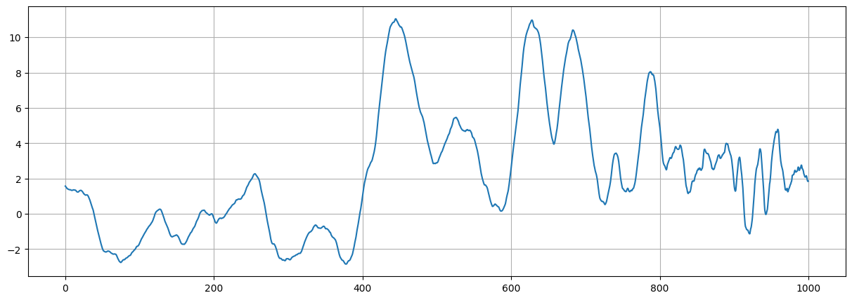
Do an unconditional simulation (reference)
[26]:
# Simulation
nreal = 1
np.random.seed(2485)
geosclassic_output = gn.geosclassicinterface.simulate(
                        cov_model_base, nx, sx, ox,
                        method='ordinary_kriging',
                        cov_model_non_stationarity_list=cov_model_non_stationarity_list,
                        nneighborMax=64,
                        nreal=nreal,
                        nproc=1, nthreads_per_proc=8)

im_ref = geosclassic_output['image']

plt.figure(figsize=(15,5))
plt.plot(im_ref.x(), im_ref.val[0,0,0])
plt.grid()
plt.show()
simulate: pre-process data done: final number of data points : 0, inequality data points: 0
simulate: computational resources: nproc = 1, nthreads_per_proc = 8, nproc_sgs_at_ineq = 8
simulate: (Step 1-3 skipped) no data
simulate: (Step 4) do sgs (1 realizations) on the grid (at cell centers) using data points at cell centers...
simulate: call `run_MPDSOMPGeosClassicSim` [1 process of 8 thread(s) (OpenMP)] ...
simulate: `run_MPDSOMPGeosClassicSim` [1 process] complete
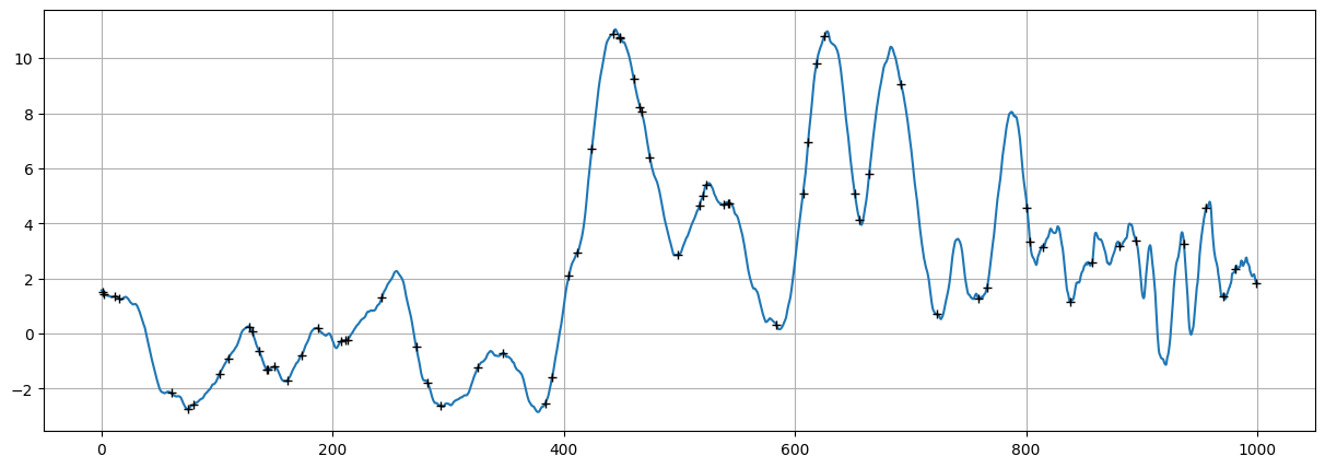
Build a non-stationary data set (1D)
The data set is defined by extracting some points from the simulation of reference.
Note: the data set should contain enough points to catch the non-stationarities.
[27]:
# Extract som points from the simulation
n = 70

# --- Choose 1. or 2. below ---
# # 1. Sampling the image
# ps = gn.img.sampleFromImage(im_ref, n, seed=234)
# # Data points and data value
# x = ps.x()
# v = ps.val[3]
# # Optionally: move points in the grid cells randomly, and add noise to values
# x = x + (np.random.random(n)-0.5)* im_ref.sx
# v = v + (np.random.random(n)-0.5)* 1.e-1

# 2. Using the function interpolating the image values
f = gn.img.Img_interp_func(im_ref, iy=0, iz=0)
np.random.seed(4253)
x = im_ref.xmin() + np.random.random(n) * (im_ref.xmax()-im_ref.xmin())
v = f(x)
# ----- #

plt.figure(figsize=(15,5))
plt.plot(im_ref.x(), im_ref.val[0,0,0])
plt.plot(x, v, '+', c='k')
plt.grid()
plt.show()
Simulation starting from a non-stationary data set in 1D and assuming “non-stationarity feature(s)” known
n: number of data pointsx: location of data points (1-dimensional array of lengthn)v: values at data points (1-dimensional array of lengthn)im_r_factor: image of the factor (multiplier)r_factorin the grid; the functionr_factor_inv_loc_func(interpolator of the inverse ofr_factorin the grid) is built from this imageim_w_factor: image of the factor (multiplier)w_factorin the grid; the functionw_factor_inv_loc_func(interpolator of the inverse ofw_factorin the grid) is built from this image
[28]:
# Set a function interpolating the inverse of the w_factor (given location)
im_tmp = gn.img.copyImg(im_w_factor)
im_tmp.val = 1.0/im_tmp.val
w_factor_inv_loc_func = gn.img.Img_interp_func(im_tmp, ind=0, iy=0, iz=0)
# -> specify iy=0, iz=0: consider only x coordinates along the "line" iy=0 and iz=0

# Set a function interpolating the inverse of the r_factor (given location)
im_tmp = gn.img.copyImg(im_r_factor)
im_tmp.val = 1.0/im_tmp.val
r_factor_inv_loc_func = gn.img.Img_interp_func(im_tmp, ind=0, iy=0, iz=0)
# -> specify iy=0, iz=0: consider only x coordinates along the "line" iy=0 and iz=0
Fitting covariance model accounting for non-stationarity
[29]:
cov_model_to_optimize = gn.covModel.CovModel1D(elem=[
        ('cubic', {'w':np.nan, 'r':np.nan}), # elementary contribution
         ], name='')

t1 = time.time()
cov_model_opt, popt = gn.covModel.covModel1D_fit(
                x, v, cov_model_to_optimize,
                w_factor_loc_func=w_factor_inv_loc_func,     # deal with non-stationarity (multiplier for weight)
                coord_factor_loc_func=r_factor_inv_loc_func, # deal with non-stationarity (multiplier for range)
                loc_m=10, # loc_m > 0: number of sub-intervals btw pair of points to estimate local factor (default 1)
                          # loc_m = 0: take factor from one point
                bounds=([   0,   0],  # min value for param. to fit
                        [ 100, 500]), # max value for param. to fit
                hmax=100, make_plot=False) # figure size for plot
t2 = time.time()
print(f'Fitting covariance model - elapsed time: {t2-t1:.4g}')

cov_model_opt
Fitting covariance model - elapsed time: 0.02022
[29]:
*** CovModel1D object ***
name = ''
number of elementary contribution(s): 1
elementary contribution 0
    type: cubic
    parameters:
        w = 8.450478582025847
        r = 52.9933842174848
*****
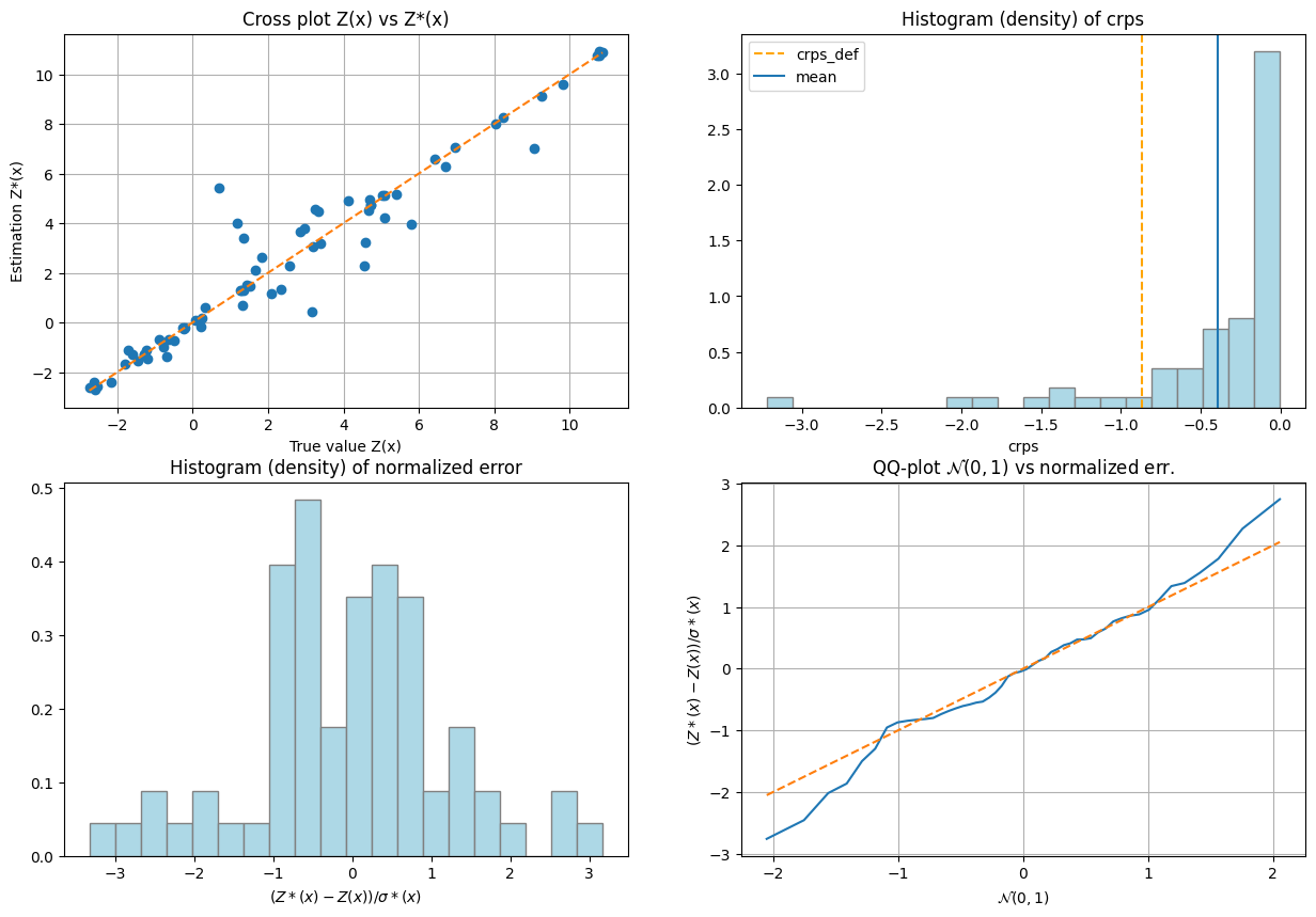
Cross-validation of covariance model by leave-one-out error
The function geone.covModel.cross_valid_loo performs a cross-validation test by leave-one-out (LOO) error.
See jupyter notebook ex_vario_analysis_data1D for more details about this function.
[30]:
# Set a function interpolating the w_factor (given location)
w_factor_loc_func = gn.img.Img_interp_func(im_w_factor, ind=0, iy=0, iz=0)
# Set a function interpolating the w_factor (given location)
r_factor_loc_func = gn.img.Img_interp_func(im_r_factor, ind=0, iy=0, iz=0)
# -> specify iy=0, iz=0: consider only x coordinates along the "line" iy=0 and iz=0

# Set list to handle non-stationarities at x
cov_model_non_stationarity_x_list = [
    ('multiply_w', w_factor_loc_func(x)),
    ('multiply_r', r_factor_loc_func(x))
]

cv_est1, cv_std1, crps1, crps_def1, pvalue1, success1 = gn.covModel.cross_valid_loo(
                                        x, v, cov_model_opt,
                                        interpolator=gn.covModel.krige,
                                        interpolator_kwargs={'method':'ordinary_kriging'},
                                        cov_model_non_stationarity_x_list=cov_model_non_stationarity_x_list,
                                        print_result=True, make_plot=True, figsize=(15,10), nbins=20)
plt.show()
----- CRPS (negative; the larger, the better) -----
   mean = -0.39
   def. = -0.8687
----- 1) "Normal law test for mean of normalized error" -----
   p-value = 0.745
   success = True (wrt significance level 0.05)
      (-> model has no reason to be rejected)
----- 2) "Chi-square test for sum of squares of normalized error" -----
   p-value = 0.002184
   success = False (wrt significance level 0.05)
      -> model should be REJECTED
----- Statistics of normalized error -----
   mean     = -0.03887 (should be close to 0)
   std      = 1.244 (should be close to 1)
   skewness = -0.03617 (should be close to 0)
   excess kurtosis = 0.5304 (should be close to 0)
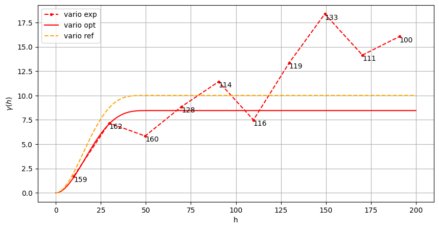
Show experimental variogram, fitted model and reference model
[31]:
hmax = 200.0

hexp, gexp, cexp = gn.covModel.variogramExp1D(x, v, hmax=hmax,
                                              w_factor_loc_func=w_factor_inv_loc_func,
                                              coord_factor_loc_func=r_factor_inv_loc_func, loc_m=10,
                                              ncla=10, make_plot=False)

plt.figure(figsize=(10,5))
gn.covModel.plot_variogramExp1D(hexp, gexp, cexp, c='red', label='vario exp')
cov_model_opt.plot_model(vario=True, hmax=hmax, c='red', label='vario opt')
cov_model_base.plot_model(vario=True, hmax=hmax, c='orange', ls='dashed', label='vario ref')
plt.legend()

plt.show()
Kriging and conditional simulations
[32]:
# Kriging
t1 = time.time() # start time
geosclassic_output = gn.geosclassicinterface.estimate(
                        cov_model_opt, nx, sx, ox,
                        x=x, v=v,
                        method='ordinary_kriging',
                        cov_model_non_stationarity_list=cov_model_non_stationarity_list,
                        nneighborMax=20,
                        nthreads=8)
t2 = time.time() # end time
print(f'Kriging - elapsed time: {t2-t1:.4g} sec')

# Retrieve kriging estimate and standard deviation
im_krig = geosclassic_output['image']
estimate: pre-process data done: final number of data points : 68, inequality data points: 0
estimate: computational resources: nthreads = 8, nproc_sgs_at_ineq = 8
estimate: (Step 1) no inequality data
estimate: (Step 2) set new dataset gathering data and inequality data locations...
estimate: (Step 3) do kriging at the center of grid cells containing at least one data point...
estimate: (Step 4) do kriging on the grid (at cell centers) using data points at cell centers...
estimate: call `run_MPDSOMPGeosClassicSim` [1 process of 8 thread(s) (OpenMP)] ...
estimate: `run_MPDSOMPGeosClassicSim` [1 process] complete
Kriging - elapsed time: 0.03166 sec
[33]:
# Simulation
nreal = 1000
np.random.seed(22131)
t1 = time.time() # start time
geosclassic_output = gn.geosclassicinterface.simulate(
                        cov_model_opt, nx, sx, ox,
                        x=x, v=v, method='ordinary_kriging',
                        cov_model_non_stationarity_list=cov_model_non_stationarity_list,
                        nneighborMax=20,
                        nreal=nreal,
                        nproc=4, nthreads_per_proc=4)
t2 = time.time() # end time
print(f'{nreal} simul. - elapsed time: {t2-t1:.4g} sec')

# Retrieve the realizations
simul = geosclassic_output['image']

# Compute mean and standard deviation (pixel-wise)
simul_mean = gn.img.imageContStat(simul, op='mean')
simul_std = gn.img.imageContStat(simul, op='std')
simulate: pre-process data done: final number of data points : 68, inequality data points: 0
simulate: computational resources: nproc = 4, nthreads_per_proc = 4, nproc_sgs_at_ineq = 16
simulate: (Step 1) no inequality data
simulate: (Step 2) set new dataset gathering data and inequality data locations...
simulate: (Step 3) do kriging at the center of grid cells containing at least one data point...
simulate: (Step 4) do sgs (1000 realizations) on the grid (at cell centers) using data points at cell centers...
simulate: call `run_MPDSOMPGeosClassicSim` [4 process(es) of 4 thread(s) (OpenMP)] ...
simulate: `run_MPDSOMPGeosClassicSim` [4 process(es)] complete
1000 simul. - elapsed time: 4.179 sec
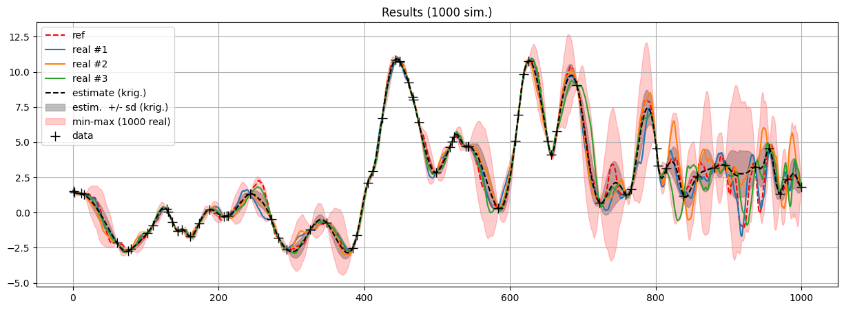
[34]:
# Plot the first simulations and the results of estimation
plt.figure(figsize=(15,5))

plt.plot(im_ref.x(), im_ref.val[0,0,0,:], c='red', ls='dashed', label='ref')

for i in range(3):
    plt.plot(simul.x(), simul.val[i,0,0,:], label='real #{}'.format(i+1))

plt.plot(im_krig.x(), im_krig.val[0,0,0,:], c='black', ls='dashed', label='estimate (krig.)')
plt.fill_between(im_krig.x(),
                 im_krig.val[0,0,0,:] - im_krig.val[1,0,0,:],
                 im_krig.val[0,0,0,:] + im_krig.val[1,0,0,:],
                 color='gray', alpha=.5, label='estim.  +/- sd (krig.)')

plt.fill_between(simul.x(), simul.val[:,0,0,:].min(axis=0), simul.val[:,0,0,:].max(axis=0),
                 color='red', alpha=.2, label='min-max ({} real)'.format(nreal))

plt.plot(x, v, '+', c='k', markersize=10, label='data') # add conditioning points

plt.grid()
plt.legend()
plt.title(f'Results ({nreal} sim.)')
plt.show()