GEONE - Variogram analysis and kriging for data in 2D (omni-directional)
Interpolate a data set in 2D, using simple or ordinary kriging. Starting from a data set in 2D, the following is done:
basic exploratory analysis: variogram cloud / variogram rose / experimental variogram
fitting a covariance / variogram model, and cross-validation (LOO error)
interpolation by ordinary kriging (OK), simple kriging (SK)
sequential gaussian simulation (SGS) based on ordinary or simple kriging
Import what is required
[1]:
import numpy as np
import matplotlib.pyplot as plt
import time

# import package 'geone'
import geone as gn
[2]:
# Show version of python and version of geone
import sys
print(sys.version_info)
print('geone version: ' + gn.__version__)
sys.version_info(major=3, minor=13, micro=7, releaselevel='final', serial=0)
geone version: 1.3.1
Preparation - build a data set in 2D
A data set in 2D is extracted from a Gaussian random field generated based on a known covariance model, called the reference model which will be considered as unknown further.
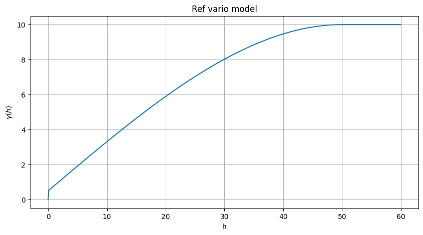
Define a (isotropic) reference covariance model in 1D (class geone.covModel.CovModel1D), used as omni-directional in 2D.
Note: see the notebook ``ex_general_multiGaussian.ipynb`` for available covariance models and examples.
[3]:
cov_model_ref = gn.covModel.CovModel1D(elem=[
    ('spherical', {'w':9.5, 'r':50}), # elementary contribution (same ranges: isotropic)
    ('nugget', {'w':0.5})                     # elementary contribution
    ], name='ref model (isotropic)')
[4]:
cov_model_ref
[4]:
*** CovModel1D object ***
name = 'ref model (isotropic)'
number of elementary contribution(s): 2
elementary contribution 0
    type: spherical
    parameters:
        w = 9.5
        r = 50
elementary contribution 1
    type: nugget
    parameters:
        w = 0.5
*****
[5]:
# Plot reference variogram model
plt.figure(figsize=(10,5))
cov_model_ref.plot_model(vario=True)
plt.title('Ref vario model')
plt.show()
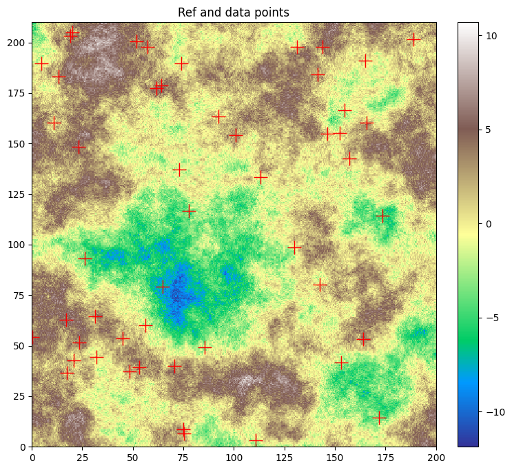
Generate a gaussian random field in 2D (see function geone.grf.grf2D), and extract data points:
n: number of data pointsx: location of data points (2-dimensional array of shape(n, 2), each row is a point)v: values at data points (1-dimensional array of lengthn)
[6]:
# Simulation grid (domain)
nx, ny = 400, 420  # number of cells
sx, sy = 0.5, 0.5  # cell unit
ox, oy = 0.0, 0.0  # origin

# Reference simulation
np.random.seed(123)
ref = gn.grf.grf2D(cov_model_ref, (nx, ny), (sx, sy), (ox, oy), nreal=1)
    # 3d-array of shape 1 x ny x nx

im_ref = gn.img.Img(nx, ny, 1, sx, sy, 1., ox, oy, 0., nv=1, val=ref) # fill image (Img class from geone.img)

# Extract n points from the reference simulation
n = 50 # number of data points
# --- Choose 1. or 2. below ---
# # 1. Sampling the image
# ps = gn.img.sampleFromImage(im_ref, n, seed=234)
# # Data points and data value
# x = np.array((ps.x(), ps.y())).T
# v = ps.val[3]
# # Optionally: move points in the grid cells randomly, and add noise to values
# x[:, 0] = x[:, 0] + (np.random.random(n)-0.5)* im_ref.sx
# x[:, 1] = x[:, 1] + (np.random.random(n)-0.5)* im_ref.sy
# v = v + (np.random.random(n)-0.5)* 1.e-1

# 2. Using the function interpolating the image values
f = gn.img.Img_interp_func(im_ref, iz=0)
np.random.seed(658)
x1 = im_ref.xmin() + np.random.random(n) * (im_ref.xmax()-im_ref.xmin())
x2 = im_ref.ymin() + np.random.random(n) * (im_ref.ymax()-im_ref.ymin())
x = np.array((x1, x2)).T
v = f(x)
# ----- #
[7]:
# Plot reference simulation and data points
plt.figure(figsize=(10,8))
gn.imgplot.drawImage2D(im_ref, cmap='terrain')
plt.plot(x[:,0], x[:,1], 'r+', markersize=15)
plt.title('Ref and data points')
plt.show()
Start from a data set in 2D
n: number of data pointsx: location of data points (2-dimensional array of shape(n, 2), each row is a point)v: values at data points (1-dimensional array of lengthn)
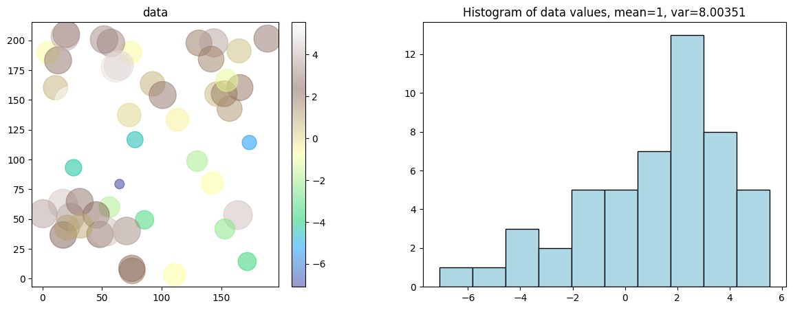
Visualise the data set and the histogram of values.
[8]:
plt.subplots(1,2,figsize=(15,5))
plt.subplot(1,2,1)
vmin, vmax = np.min(v), np.max(v) # min and max of data values
smin, smax = 100, 1000            # min and max size of points on plot
plot = plt.scatter(x[:,0], x[:,1], c=v, s=smin+(v-vmin)/(vmax-vmin)*(smax-smin), alpha=0.5, cmap='terrain')
gn.customcolors.add_colorbar(plot)
plt.axis('equal')
plt.title('data')

plt.subplot(1,2,2)
plt.hist(v, color='lightblue', edgecolor='black')
plt.title('Histogram of data values, mean={:.2g}, var={:2g}'.format(np.mean(v), np.var(v)))
plt.show()
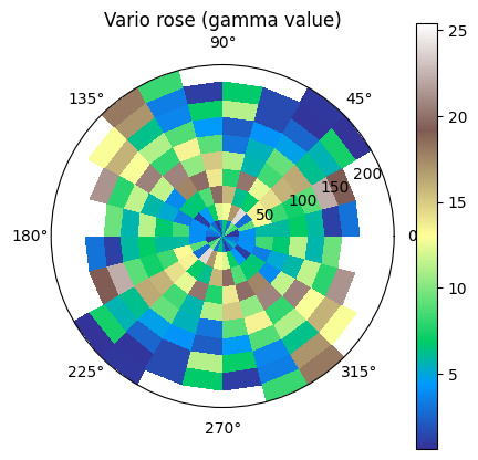
Variogram rose
The function geone.covModel.variogramExp2D_rose shows an experimental variogram for a data set in 2D in the form of a rose plot, i.e. the lags vectors between the pairs of data points are divided in classes according to length (radius) and angle from the x-axis counter-clockwise (warning: opposite sense to the sense given by angle in definition of a covariance model in 2D).
The keyword argument r_max allows to specify a maximal length of 2D-lag vector between a pair of data points for being integrated in the variogram rose plot. The number of classes for radius (length) can be specified by the keyword argument r_ncla, and the number of classes for angle for half of the whole disk (rose plot is symmetric with respect to the origin) can be specified by the keyword argument phi_ncla.
This function can be useful to check a possible anisotropy.
[9]:
gn.covModel.variogramExp2D_rose(x, v, figsize=(5,5))
plt.show()
/home/julien/miniconda3/envs/py313/lib/python3.13/site-packages/numpy/_core/fromnumeric.py:3860: RuntimeWarning: Mean of empty slice.
  return _methods._mean(a, axis=axis, dtype=dtype,
/home/julien/miniconda3/envs/py313/lib/python3.13/site-packages/numpy/_core/_methods.py:144: RuntimeWarning: invalid value encountered in scalar divide
  ret = ret.dtype.type(ret / rcount)
For plotting a variogram rose in a multiple axes figure, proceed as follows.
[10]:
fig = plt.figure(figsize=(15,5))

fig.add_subplot(1,2,1, projection='polar')
gn.covModel.variogramExp2D_rose(x, v, set_polar_subplot=False)

ax = fig.add_subplot(1,2,2, projection='polar')
gn.covModel.variogramExp2D_rose(x, v, r_max=100, set_polar_subplot=False)

plt.show()
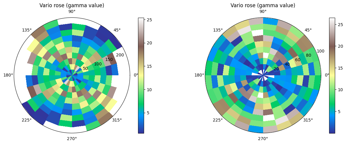
As no anisotropy is visible, an omni-directional covariance / variogram model could be used.
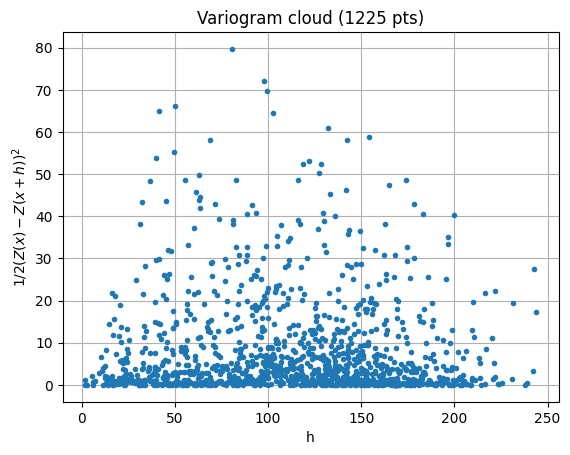
Omni-directional variogram cloud
The function geone.covModel.variogramCloud1D is used (see jupyter notebook ex_vario_analysis_data1D).
[11]:
h, g, npair = gn.covModel.variogramCloud1D(x, v)
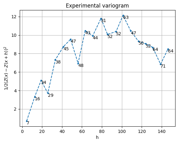
Omni-directional experimental variogram
The function geone.covModel.variogramExp1D is used (see jupyter notebook ex_vario_analysis_data1D).
[12]:
hexp, gexp, cexp = gn.covModel.variogramExp1D(x, v)
# hexp, gexp, cexp = gn.covModel.variogramExp1D(x, v, variogramCloud=(g, h, npair)) # equivalent (x, v not used)

[13]:
hexp, gexp, cexp = gn.covModel.variogramExp1D(x, v, hmax=150, ncla=20)
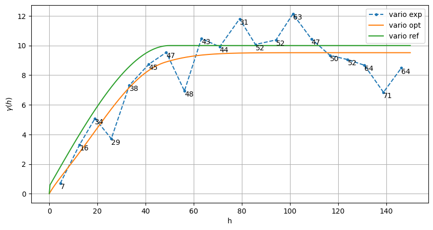
Omni-directional model fitting
The function geone.covModel.covModel1D_fit is used to fit a covariance model in 1D (class geone.covModel.CovModel1D) (see jupyter notebook ex_vario_analysis_data1D).
[14]:
cov_model_to_optimize = gn.covModel.CovModel1D(
    elem=[('gaussian',    {'w':np.nan, 'r':np.nan}), # elementary contribution
          ('spherical',   {'w':np.nan, 'r':np.nan}), # elementary contribution
          ('exponential', {'w':np.nan, 'r':np.nan}), # elementary contribution
          ('nugget',      {'w':np.nan})              # elementary contribution
         ], name='')

hmax = 150
cov_model_opt, popt = gn.covModel.covModel1D_fit(x, v, cov_model_to_optimize, hmax=hmax,
                        bounds=([ 0,   0,  0,   0,  0,   0,  0],  # min value for param. to fit
                                [20, 150, 20, 150, 20, 150, 20]), # max value for param. to fit
                        make_plot=False)
plt.figure(figsize=(10,5))
gn.covModel.plot_variogramExp1D(hexp, gexp, cexp, label='vario exp')
cov_model_opt.plot_model(vario=True, hmax=hmax, label='vario opt') # cov. model in 1D
cov_model_ref.plot_model(vario=True, hmax=hmax, label='vario ref') # cov. model in 1D
plt.legend()
plt.show()
cov_model_opt
[14]:
*** CovModel1D object ***
name = ''
number of elementary contribution(s): 4
elementary contribution 0
    type: gaussian
    parameters:
        w = 4.275801892436917
        r = 60.59914771211239
elementary contribution 1
    type: spherical
    parameters:
        w = 4.811228456216264
        r = 48.17956254410442
elementary contribution 2
    type: exponential
    parameters:
        w = 0.43072653821403795
        r = 9.896047971113909
elementary contribution 3
    type: nugget
    parameters:
        w = 0.0002605124942035417
*****
Cross-validation of covariance model by leave-one-out error
The function geone.covModel.cross_valid_loo performs a cross-validation test by leave-one-out (LOO) error.
For a given a data set (in 2D) and a covariance model in 1D, this latter defines an omni-directional covariance model.
See jupyter notebook ex_vario_analysis_data1D for more details about this function.
[15]:
# Interpolation by simple kriging
cv_est1, cv_std1, crps1, crps_def1, pvalue1, success1 = gn.covModel.cross_valid_loo(
                                        x, v, cov_model_opt,
                                        interpolator=gn.covModel.krige,
                                        interpolator_kwargs={'method':'ordinary_kriging'},
                                        print_result=True, make_plot=True, figsize=(15,10), nbins=20)
plt.show()
----- CRPS (negative; the larger, the better) -----
   mean = -1.334
   def. = -0.6611
----- 1) "Normal law test for mean of normalized error" -----
   p-value = 0.6322
   success = True (wrt significance level 0.05)
      (-> model has no reason to be rejected)
----- 2) "Chi-square test for sum of squares of normalized error" -----
   p-value = 0.08793
   success = True (wrt significance level 0.05)
      (-> model has no reason to be rejected)
----- Statistics of normalized error -----
   mean     = 0.06768 (should be close to 0)
   std      = 1.129 (should be close to 1)
   skewness = -0.1555 (should be close to 0)
   excess kurtosis = -0.7574 (should be close to 0)

If one test failed (or if the covariance model does not display the desired shape), the covariance model should be rejected and the search for a convenient covariance model be pursued.
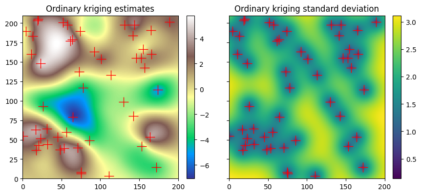
Data interpolation by (simple or ordinary) kriging: function geone.covModel.krige
See notebook ex_vario_analysis_data1D_1.ipynb.
[16]:
# Define points xu where to interpolate
# ... location of the 2D-grid used to build the data set (but it could be different)
xcu = ox + (np.arange(nx)+0.5)*sx # x-coordinates of points
ycu = oy + (np.arange(ny)+0.5)*sy # y-coordinates of points
xxcu, yycu = np.meshgrid(xcu, ycu)
xu = np.array((xxcu.reshape(-1), yycu.reshape(-1))).T # 2-dimensional array of shape nx*ny x 2

# Ordinary kriging
t1 = time.time() # start time
vu, vu_std = gn.covModel.krige(x, v, xu, cov_model_opt, method='ordinary_kriging', use_unique_neighborhood=True)
# vu:     1-dimensional array, kriging estimates at location xu
# vu_std: 1-dimensional array, kriging standard deviation at location xu
t2 = time.time() # end time
print(f'Elapsed time: {t2-t1:.4g} sec')

# Fill image (Img class from geone.img) for view
#   variable 0: kriging estimates
#   variable 1: kriging standard deviation
im_krig = gn.img.Img(nx, ny, 1, sx, sy, 1., ox, oy, 0., nv=2, val=np.array((vu, vu_std)))

# Plot
plt.subplots(1,2, figsize=(10,5), sharey=True)

plt.subplot(1,2,1)
gn.imgplot.drawImage2D(im_krig, iv=0, cmap='terrain', title='Ordinary kriging estimates')
plt.plot(x[:,0], x[:,1], 'r+', markersize=15)

plt.subplot(1,2,2)
gn.imgplot.drawImage2D(im_krig, iv=1, cmap='viridis', title='Ordinary kriging standard deviation')
plt.plot(x[:,0], x[:,1], 'r+', markersize=15)

plt.show()
Elapsed time: 0.3894 sec
[17]:
# Define points xu where to interpolate
# ... location of the 2D-grid used to build the data set (but it could be different)
xcu = ox + (np.arange(nx)+0.5)*sx # x-coordinates of points
ycu = oy + (np.arange(ny)+0.5)*sy # y-coordinates of points
xxcu, yycu = np.meshgrid(xcu, ycu)
xu = np.array((xxcu.reshape(-1), yycu.reshape(-1))).T # 2-dimensional array of shape nx*ny x 2

# Simple kriging
t1 = time.time() # start time
vu, vu_std = gn.covModel.krige(x, v, xu, cov_model_opt, method='simple_kriging', use_unique_neighborhood=True)
# vu:     1-dimensional array, kriging estimates at location xu
# vu_std: 1-dimensional array, kriging standard deviation at location xu
t2 = time.time() # end time
print(f'Elapsed time: {t2-t1:.4g} sec')

# Fill image (Img class from geone.img) for view
#   variable 0: kriging estimates
#   variable 1: kriging standard deviation
im_krig = gn.img.Img(nx, ny, 1, sx, sy, 1., ox, oy, 0., nv=2, val=np.array((vu, vu_std)))

# Plot
plt.subplots(1,2, figsize=(10,5), sharey=True)

plt.subplot(1,2,1)
gn.imgplot.drawImage2D(im_krig, iv=0, cmap='terrain', title='Simple kriging estimates')
plt.plot(x[:,0], x[:,1], 'r+', markersize=15)

plt.subplot(1,2,2)
gn.imgplot.drawImage2D(im_krig, iv=1, cmap='viridis', title='Simple kriging standard deviation')
plt.plot(x[:,0], x[:,1], 'r+', markersize=15)

plt.show()
Elapsed time: 0.3846 sec

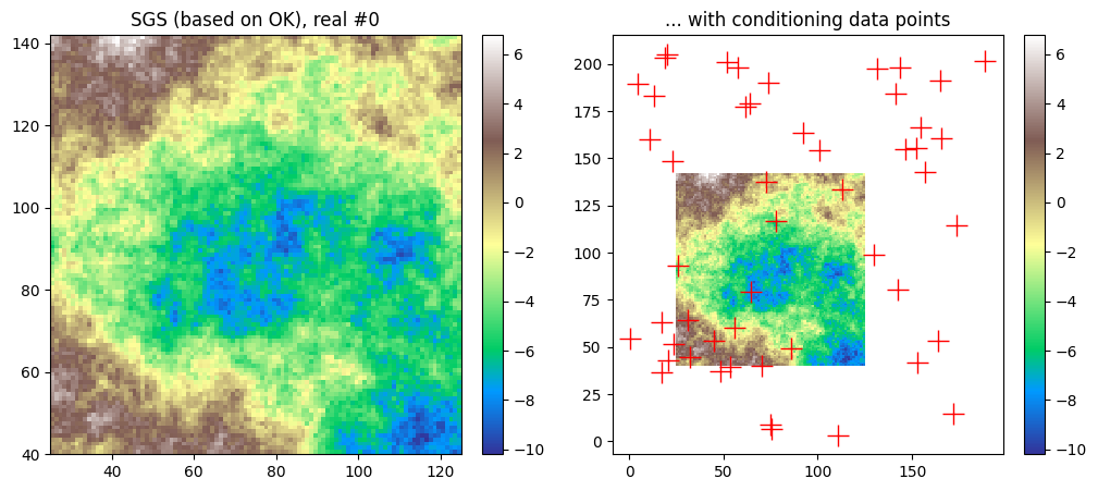
Simulation based on simple or ordinary kriging: function geone.covModel.sgs
See notebook ex_vario_analysis_data1D_1.ipynb.
[18]:
# Define points xu where to simulate
# take less points for simulation
sim_nx, sim_ny = 100, 102 # less points
sim_sx, sim_sy = 2*sx, 2*sy # coarser resolution
sim_ox, sim_oy = 25., 40.
sim_xcu = sim_ox + (np.arange(sim_nx)+0.5)*sim_sx # x-coordinates of points
sim_ycu = sim_oy + (np.arange(sim_ny)+0.5)*sim_sy # y-coordinates of points
sim_xxcu, sim_yycu = np.meshgrid(sim_xcu, sim_ycu)
sim_xu = np.array((sim_xxcu.reshape(-1), sim_yycu.reshape(-1))).T # 2-dimensional array of with two columns

# SGS based on ordinary kriging
nreal = 1
np.random.seed(321)
t1 = time.time() # start time
sim_vu = gn.covModel.sgs(x, v, sim_xu, cov_model_opt, method='ordinary_kriging', nreal=nreal)
# sim_vu:   2-dimensional array of shape (nreal, sim_xu.shape[0]), each row is a realization
#           (simulated values at locations sim_xu)
t2 = time.time() # end time
print(f'{nreal} simul. - elapsed time: {t2-t1:.4g} sec')

# Fill image (Img class from geone.img) for view
im_sim = gn.img.Img(sim_nx, sim_ny, 1, sim_sx, sim_sy, 1., sim_ox, sim_oy, 0., nv=nreal, val=sim_vu)

# Plot
plt.subplots(1,2, figsize=(12,5))

plt.subplot(1,2,1)
gn.imgplot.drawImage2D(im_sim, iv=0, cmap='terrain', title='SGS (based on OK), real #0')
#plt.plot(x[:,0], x[:,1], 'r+', markersize=15)

plt.subplot(1,2,2)
gn.imgplot.drawImage2D(im_sim, iv=0, cmap='terrain', title='... with conditioning data points')
plt.plot(x[:,0], x[:,1], 'r+', markersize=15)

plt.show()
1 simul. - elapsed time: 4.411 sec
Kriging estimation and simulation in a grid
The function above (gn.covModel.krige and gn.covModel.sgs[_mp]) should not be used for kriging and SGS in a regular grid. Use the dedicated functions (much faster):
geone.geosclassicinterface.estimate: estimation (kriging) in a gridgeone.geosclassicinterface.simulate: simulation (SGS) in a gridgeone.grf.krige<d>D: estimation (kriging) in a<d>-dimensional gridgeone.grf.grf<d>D: simulation (SGS) in a<d>-dimensional grid
Note: the functions of the module ``geone.grf`` are based on “Fast Fourier Transform” and allow for simple kriging only, and do not handle error on data or inequality data.
Note: the function ``geone.multiGaussian.multiGaussianRun`` can be used as a wrapper to run the functions above.
See notebook ex_vario_analysis_data1D_1.ipynb.
Examples
Estimation using the function geone.covModel.krige
[19]:
t1 = time.time()
vu, vu_std = gn.covModel.krige(x, v, xu, cov_model_opt, method='simple_kriging', use_unique_neighborhood=True)
t2 = time.time()
print('Elapsed time: {:.2g} sec'.format(t2-t1))
Elapsed time: 0.43 sec
Estimation using the function geone.grf.krige2D
Via the function geone.multiGaussian.multiGaussianRun, with keyword arguments mode='estimation', algo='fft'.
[20]:
t1 = time.time()
im_grf = gn.multiGaussian.multiGaussianRun(
                cov_model_opt, (nx, ny), (sx, sy), (ox, oy),
                x=x, v=v,
                mode='estimation', algo='fft', output_mode='img')
# # Or:
# vu_grf, vu_std_grf = gn.grf.krige2D(cov_model_opt, (nx, ny), (sx, sy), (ox, oy),
#                 cov_model_opt, (nx, ny), (sx, sy), (ox, oy),
#                 x=x, v=v)
# im_grf = gn.img.Img(nx, ny, 1, sx, sy, 1., ox, oy, 0., nv=2, val=np.array((vu_grf, vu_std_grf)))
t2 = time.time()
print('Elapsed time: {:.2g} sec'.format(t2-t1))
krige2D: compute circulant embedding...
krige2D: embedding dimension: 1024 x 1024
krige2D: compute FFT of circulant matrix...
krige2D: compute covariance matrix (rAA) for conditioning locations...
krige2D: compute covariance matrix (rBA) for non-conditioning / conditioning locations...
krige2D: compute rBA * rAA^(-1)...
krige2D: compute kriging estimates...
krige2D: compute kriging standard deviation ...
Elapsed time: 0.57 sec
Estimation using the function geone.geosclassicinterface.estimate
Via the function geone.multiGaussian.multiGaussianRun, with keyword arguments mode='estimation', algo='classic'.
[21]:
t1 = time.time()
im_gci = gn.multiGaussian.multiGaussianRun(
                cov_model_opt, (nx, ny), (sx, sy), (ox, oy),
                x=x, v=v,
                mode='estimation', algo='classic', output_mode='img',
                method='simple_kriging', use_unique_neighborhood=True,
                nthreads=8)
# # Or:
# estim_gci = gn.geosclassicinterface.estimate(
#                 cov_model_opt, (nx, ny), (sx, sy), (ox, oy),
#                 x=x, v=v,
#                 method='simple_kriging', use_unique_neighborhood=True)
# im_gci = estim_gci['image']
t2 = time.time()
print('Elapsed time: {:.2g} sec'.format(t2-t1))
estimate: pre-process data done: final number of data points : 50, inequality data points: 0
estimate: computational resources: nthreads = 8, nproc_sgs_at_ineq = 8
estimate: (Step 1) no inequality data
estimate: (Step 2) set new dataset gathering data and inequality data locations...
estimate: (Step 3) do kriging at the center of grid cells containing at least one data point...
estimate: (Step 4) do kriging on the grid (at cell centers) using data points at cell centers...
estimate: call `run_MPDSOMPGeosClassicSim` [1 process of 8 thread(s) (OpenMP)] ...
estimate: `run_MPDSOMPGeosClassicSim` [1 process] complete
Elapsed time: 3.4 sec
Plot results of estimation
[22]:
# Fill images (Img class from geone.img) for view
#   variable 0: kriging estimates
#   variable 1: kriging standard deviation
im_krig = gn.img.Img(nx, ny, 1, sx, sy, 1., ox, oy, 0., nv=2, val=np.array((vu, vu_std)))

# Plot
plt.subplots(2,3, figsize=(16,10), sharex=True, sharey=True)

plt.subplot(2,3,1)
gn.imgplot.drawImage2D(im_krig, iv=0, cmap='terrain', title="Krig. est. 'gn.covModel.krige'")
plt.plot(x[:,0], x[:,1], 'r+', markersize=15)

plt.subplot(2,3,2)
gn.imgplot.drawImage2D(im_grf, iv=0, cmap='terrain', title="Krig. est. 'gn.grf.krige2D'")
plt.plot(x[:,0], x[:,1], 'r+', markersize=15)

plt.subplot(2,3,3)
gn.imgplot.drawImage2D(im_gci, iv=0, cmap='terrain', title="Krig. est. 'gn.geosclassicinterface.estimate'")
plt.plot(x[:,0], x[:,1], 'r+', markersize=15)

plt.subplot(2,3,4)
gn.imgplot.drawImage2D(im_krig, iv=1, cmap='viridis', title="Krig. std 'gn.covModel.krige'")
plt.plot(x[:,0], x[:,1], 'r+', markersize=15)

plt.subplot(2,3,5)
gn.imgplot.drawImage2D(im_grf, iv=1, cmap='viridis', title="Krig. std 'gn.grf.krige2D'")
plt.plot(x[:,0], x[:,1], 'r+', markersize=15)

plt.subplot(2,3,6)
gn.imgplot.drawImage2D(im_gci, iv=1, cmap='viridis', title="Krig. std 'gn.geosclassicinterface.estimate'")
plt.plot(x[:,0], x[:,1], 'r+', markersize=15)

plt.show()
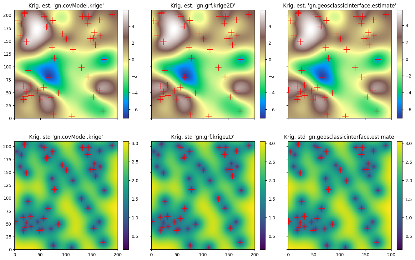
[23]:
print("Peak-to-peak estimation 'gn.covModel.krige - gn.grf.krige2D'                     = {}".format(np.ptp(im_krig.val[0] - im_grf.val[0])))
print("Peak-to-peak estimation 'gn.covModel.krige - gn.geosclassicinterface.estimate2D' = {}".format(np.ptp(im_krig.val[0] - im_gci.val[0])))
print("Peak-to-peak estimation 'gn.grf.krige2D    - gn.geosclassicinterface.estimate2D' = {}".format(np.ptp(im_grf.val[0] - im_gci.val[0])))
print("Peak-to-peak st. dev.   'gn.covModel.krige - gn.grf.krige2D'                     = {}".format(np.ptp(im_krig.val[1] - im_grf.val[1])))
print("Peak-to-peak st. dev.   'gn.covModel.krige - gn.geosclassicinterface.estimate2D' = {}".format(np.ptp(im_krig.val[1] - im_gci.val[1])))
print("Peak-to-peak st. dev.   'gn.grf.krige2D    - gn.geosclassicinterface.estimate2D' = {}".format(np.ptp(im_grf.val[1] - im_gci.val[1])))
Peak-to-peak estimation 'gn.covModel.krige - gn.grf.krige2D'                     = 0.30737661539222083
Peak-to-peak estimation 'gn.covModel.krige - gn.geosclassicinterface.estimate2D' = 0.5367769238152618
Peak-to-peak estimation 'gn.grf.krige2D    - gn.geosclassicinterface.estimate2D' = 0.2612659314695387
Peak-to-peak st. dev.   'gn.covModel.krige - gn.grf.krige2D'                     = 0.25202512381313064
Peak-to-peak st. dev.   'gn.covModel.krige - gn.geosclassicinterface.estimate2D' = 0.2669320270950835
Peak-to-peak st. dev.   'gn.grf.krige2D    - gn.geosclassicinterface.estimate2D' = 0.13048658726838092
Conditional simulation using the function geone.grf.grf2D
Via the function geone.multiGaussian.multiGaussianRun, with keyword arguments mode='simulation', algo='fft'.
[24]:
np.random.seed(293)

t1 = time.time()
nreal = 100
im_sim_grf = gn.multiGaussian.multiGaussianRun(
                    cov_model_opt, (nx, ny), (sx, sy), (ox, oy),
                    x=x, v=v,
                    mode='simulation', algo='fft', output_mode='img',
                    nreal=nreal)
# # Or:
# sim_grf = gn.grf.grf2D(
#                     cov_model_opt, (nx, ny), (sx, sy), (ox, oy),
#                     x=x, v=v,
#                     nreal=nreal)
# im_sim_grf = gn.img.Img(nx, ny, 1, sx, sy, 1., ox, oy, 0., nv=nreal, val=sim_grf)
t2 = time.time()
print('Elapsed time: {:.2g} sec'.format(t2-t1))
grf2D: do preliminary computation...
grf2D: compute circulant embedding...
grf2D: embedding dimension: 1024 x 1024
grf2D: compute FFT of circulant matrix...
grf2D: treatment of conditioning data...
grf2D: compute covariance matrix (rAA) for conditioning locations...
grf2D: compute index in the embedding grid for non-conditioning / conditioning locations...
Elapsed time: 11 sec
Conditional simulation using the function geone.geosclassicinterface.simulate
Via the function geone.multiGaussian.multiGaussianRun, with keyword arguments mode='simulation', algo='classic', and specifying the computational resources (nproc and nthreads_per_proc).
[25]:
np.random.seed(293)

t1 = time.time()
nreal = 100
im_sim_gci = gn.multiGaussian.multiGaussianRun(
                    cov_model_opt, (nx, ny), (sx, sy), (ox, oy),
                    x=x, v=v,
                    mode='simulation', algo='classic', output_mode='img',
                    method='simple_kriging',
                    nreal=nreal,
                    nproc=2, nthreads_per_proc=4)
# # Or:
# sim_gci = gn.geosclassicinterface.simulate(
#                     cov_model_opt, (nx, ny), (sx, sy), (ox, oy),
#                     x=x, v=v,
#                     method='simple_kriging',
#                     nreal=nreal,
#                     nproc=4, nthreads_per_proc=4)
# im_sim_gci = sim_gci['image']
t2 = time.time()
print('Elapsed time: {:.2g} sec'.format(t2-t1))
simulate: pre-process data done: final number of data points : 50, inequality data points: 0
simulate: computational resources: nproc = 2, nthreads_per_proc = 4, nproc_sgs_at_ineq = 8
simulate: (Step 1) no inequality data
simulate: (Step 2) set new dataset gathering data and inequality data locations...
simulate: (Step 3) do kriging at the center of grid cells containing at least one data point...
simulate: (Step 4) do sgs (100 realizations) on the grid (at cell centers) using data points at cell centers...
simulate: call `run_MPDSOMPGeosClassicSim` [2 process(es) of 4 thread(s) (OpenMP)] ...
simulate: `run_MPDSOMPGeosClassicSim` [2 process(es)] complete
Elapsed time: 19 sec
Plot some realizations and compare to the reference simulation
[26]:
# min and max over all real and ref. sim
im_vmin = min(np.min(im_sim_grf.vmin()), np.min(im_sim_gci.vmin()), im_ref.vmin()[0])
im_vmax = max(np.max(im_sim_grf.vmax()), np.min(im_sim_gci.vmax()), im_ref.vmax()[0])

# Plot
plt.subplots(2,3, figsize=(16,10), sharex=True, sharey=True)

plt.subplot(2,3,1)
gn.imgplot.drawImage2D(im_ref, cmap='terrain', vmin=im_vmin, vmax=im_vmax, title='Ref. sim')
plt.plot(x[:,0], x[:,1], 'r+', markersize=15)

plt.subplot(2,3,2)
gn.imgplot.drawImage2D(im_sim_grf, iv=0, cmap='terrain', title="Real. #0 'gn.grf.grf2D'")
plt.plot(x[:,0], x[:,1], 'r+', markersize=15)

plt.subplot(2,3,3)
gn.imgplot.drawImage2D(im_sim_gci, iv=0, cmap='terrain', title="Real. #0 'gci.simulate'")
plt.plot(x[:,0], x[:,1], 'r+', markersize=15)

plt.subplot(2,3,4)
plt.axis('off')

plt.subplot(2,3,5)
gn.imgplot.drawImage2D(im_sim_grf, iv=1, cmap='terrain', title="Real. #1 'gn.grf.grf2D'")
#plt.plot(x[:,0], x[:,1], 'r+', markersize=15)

plt.subplot(2,3,6)
gn.imgplot.drawImage2D(im_sim_gci, iv=1, cmap='terrain', title="Real. #1 'gci.simulate'")
#plt.plot(x[:,0], x[:,1], 'r+', markersize=15)

plt.show()
Note that the nugget weight in the optimal covariance model found is close to zero, whereas in the reference covariance model, its value is 0.5. As a matter of fact, the reference simulation above is a bit more “noisy”. To ensure a larger nugget in the optimal covariance model, a minimal bound can be set accordingly for this parameter and passed to the function geone.covModel.covModel1D_fit.